Motivation
Ever since I took control of my own running data, I’ve been gradually adding features to reduce my reliance on Strava/Garmin’s analytics and have it all custom instead for my training purposes. One bit of analysis I’ve always wanted to do is model my fitness with the objective of providing accurate race time predictions (or at least more accurate than Garmin’s which I’m wildly sceptical of - I’ve no idea how accurate Strava’s are as I don’t pay for premium).
Modelling fitness isn’t too hard - you can simply look at your pace per heart rate for a rough guide - however, predicting race times is a lot more involved. I’ve had several attempts in the past but I’ve always gotten myself trapped in a vicious cycle of how to untangle the two scenarios of “my heart rate was high because I’m unfit” from “my heart rate was high because I was racing”, and my models always ended up with structural problems as a result. I didn’t have the time or motivation to spend a lot of effort on improving my Stan modelling as it’s not a skill I use too often, but I still had this nagging feeling at the back of my head that I wanted to complete this analysis.
When LLMs really started to become ready for everyday use (let’s say Opus 5.5) I thought this could be an interesting case study. I was well familiar with how these models performed in small well-defined and verifiable tasks in general software design, but this is a more open-ended problem that involves understanding the data and the problem context, statistical modelling of time-series data, Bayesian modelling, and Stan syntax as well as understanding common structural issues with Stan models.
In the end, this first attempt at vibe-analysis worked very well and produced a model that did exactly what I want, and even more importantly it taught me a lot about statistical modelling along the way.
I’m not using AI to write this post, as I am perfectly capable of writing long-winded rambling text without artificial assistance.
Data
The dataset comprises 1,410 runs from July 2018 to September 2026, with GPS and heart rate (on nearly all runs). The majority of the runs are at easy pace with some speedwork sessions mixed in. I’ve only actually run 5 official races in that time, plus 17 time trials/park runs, which is a limitation from a model validation perspective. In total then there were 22 runs marked as ‘race’ using a combination of regex parsing and mannual annotation. Also muddying the waters are the 72 runs where I was pushing a running stroller adding extra load.
Effort and training load
Throughout, heart rate $h$ is converted into a fraction of heart-rate reserve, termed effort, where $e=0$ at resting heart rate and $e=1$ at maximum heart rate.
$$e = (h - h_\text{rest}) / (h_\text{max} - h_\text{rest})$$
The training load from each run is quantified using the Heart Rate Stress Score (HRSS), which weights time at high heart rate exponentially more than time at low heart rate, scaled so that an hour at threshold heart rate scores 100.
TODO Put this as an equation rather than R code
Show the code
hrss <- function(hr, time, hr_max = 194, hr_rest = 52, hr_thr = 170) {
  e  <- pmax((hr - hr_rest) / (hr_max - hr_rest), 0)       # effort, clipped at 0
  dt <- c(0, diff(as.numeric(time))) / 60                  # minutes since last sample
  dt[dt > 5] <- 0                                          # ignore pauses
  e_thr <- (hr_thr - hr_rest) / (hr_max - hr_rest)
  100 * sum(dt * 0.64 * e * exp(1.92 * e)) / (60 * 0.64 * e_thr * exp(1.92 * e_thr))
}
Initial attempts: Banister models with Sonnet 4.6 (v1-4)
v1: Heart rate at a target pace
The first set of models were built in July 2026 using Sonnet 4.6 via Copilot. I don’t have the exact prompt to hand but I essentially sketched out the task and the dataset and asked Claude to design a model in Stan. It produced v1, which models the heart rate at a 6:00/km pace. It does this via a 2-step process of fitting a regression within each run of heart rate against pace, predicting the heart rate at the target pace and using that as the fitness measure.
$$h_{r,i+4} = \alpha_r + \beta_r\, p_{r,i} + \delta_r\,(t_{r,i} - \bar{t}_r) + \epsilon_{r,i} \qquad \epsilon_{r,i} \sim \mathcal{N}(0, \sigma_r)$$
where for a given run $r$ and timepoint $i$, $p_{r, i}$ is the measured pace (in minutes/km), $h_{r, i+4}$ is the heart rate 4 samples later (to account for the lag between pace and heart rate), $t_{r, i}$ is the time since the start, and $\bar t_r$ its average. $\alpha$ is the intercept, here indicating the heart rate when stationary (0 pace) and halfway through the run, $\beta$ is the increase in heart rate for a 1 minute increase in pace, and $\delta$ quantifies the heart rate drift throughout a run. All three of these parameters are estimated via ordinary least squares which can then be used to estimate the heart rate at 6 min/km pace:
$$y_r = \hat \alpha_r + 6\hat \beta_r$$
$y_r$ is then treated as the performance value at the point of run $r$ and is then incorporated into the long-term fitness dynamics provided by the Banister impulse-response model (BIRM, Banister et al., 1975), which decomposes each day’s training load $L_d$ into a slowly decaying fitness $F$ and a quickly decaying fatigue $G$:
$$y_r \sim \mathcal{N}\left( \mu_0 - b_F F_d + b_G G_d,\ \sqrt{s_r^2 + \sigma^2} \right)$$ $$F_d = F_{d-1}\, e^{-1/\tau_F} + k_F L_d$$ $$G_d = G_{d-1}\, e^{-1/\tau_G} + k_G L_d$$
Performance is then the difference between fitness and fatigue, so a hard session will make you faster once the fatigue has decayed but before fitness does.
v2: Latent effort
I didn’t like this approach as the 6:00/km felt somewhat arbitrary and not representative of race pace. Furthermore, the regression step required discarding a huge amount of runs which didn’t have sufficient variation to extrapolate to the target pace. And the final issue with this model is that it doesn’t directly provide a means for predicting pace at a given race distance - that still remains to be extrapolated from the output heart rate at 6:00/km.
I asked Claude to instead try and develop the idea I’d had in my head of a latent ‘effort’ that affects both heart rate and pace separately and it came up with the model below:
$$ \overline{h}_r \sim \mathcal{N}\left( h_{\text{rest}} + e_r (h_{\max} - h_{\text{rest}}) + \gamma D_r,\ \sigma_h \right), \quad $$ $$ \overline{p}_r \sim \mathcal{N}\left( \mu + b_e (0.75 - e_r) - b_F F_d + b_G G_d,\ \sigma_p \right), $$
where $\overline{h}_r$ is the average heart rate and $D_r$ the distance for run $r$ respectively. $e_r$ is the latent ‘effort’ variable that attempts to quantify how much effort I put in in this run as the fraction of my heart rate reserve I reached ($e_r = 1$ denotes running at maximum heart rate and $e_r = 0$ is at rest).
The latent $e_r$ is then used in the second equation where $\overline{p}_r$ represents the average pace for run $r$, $F_d$ and $G_d$ are the Banister terms from before, and $\mu$ is the pace at effort 0.75 if there was no fitness or fatigue. 0.75 was chosen to centre effort so $\mu$ was interpretable at an average run effort.
However, with there being only 1 noisy measurement to estimate each $e_r$ from, and $e_r$ attempting to quantify two separate ideas: firstly how much effort I was putting in, and secondly how efficient my heart rate translates to pace, this model failed to sample. NUTS never converged with a max $\hat{R} = 1.31$. This is generally what happens with many of my Stan models - I get carried away with adding latent variables everywhere and produce an unidentifiable mess.
v3: Measured effort
To overcome the identifiability issue I next asked Claude to calculate effort directly from heart rate and incorporate it into the model as data, not a parameter. Otherwise the likelihood remained unchnaged from the previous version, now vastly simplified without the heart rate model.
$$ e_r = \frac{\overline{h}_r - h_{\text{rest}}}{h_{\text{max}} - h_{\text{rest}}} $$ $$ \overline{p}_r \sim \mathcal{N}\left( \mu + b_e (\bar e - e_r) - b_F F_d + b_G G_d,\ \sigma_p \right) $$
Unsurprisingly this sampled far better, with maximum $\hat{R}=1.013$, although it had 118 divergences. These were caused by a structural problem that later versions of Claude pointed out instantly: the product of two parameters $k_F b_F$ affects the predicted pace and makes these parameters unidentifiable (this is also true for $k_G b_G$). Let’s look at this in more detail. The predicted pace is a function of $b_F F_d$, which expands to $b_F (F_{d-1}\, e^{-1/\tau_F} + k_F L_d)$. This means that the sampler can’t differentiate a scenario of low $b_F$ and high $k_F$ (fitness doesn’t effect pace, training greatly increases fitness) from high $b_F$ and low $k_F$ (fitness has a big impact on pace, training doesn’t increase fitness) and it gets stuck.
v4: Separated races and added temperature effect
Another issue with v3 was that it still places a lot of emphasis on the heart rate measurement, yet many factors influence heart rate beyond how fast you are running. Temperature is a big one, as well as current fatigue levels or general health. Furthermore, the model treats all runs the same, yet we have further information from races where we know we run flat out far beyond what is done in a training race so the model both breaks down, and we have useful data to pin against.
v4 then added the daily mean temperature on the day of run $r$ $T_r$ along with its median $\bar T$, provides races their own variance (lower than training runs as races will always be flat out), and replaces the measured effort with a curve for races.
$e = 0.967 - 0.063 \log D$, where $D$ is the race distance.
$$ e^*_r = \begin{cases} 0.967 - 0.063 \log D_r & \text{race} \\ e_r & \text{otherwise} \end{cases} $$ $$ \overline{p}_r \sim \mathcal{N}\left( \mu + b_e (\bar e - e^*_r) + b_T (T_r - \bar T) - b_F F_d + b_G G_d,\ \sigma_{[r]} \right) $$
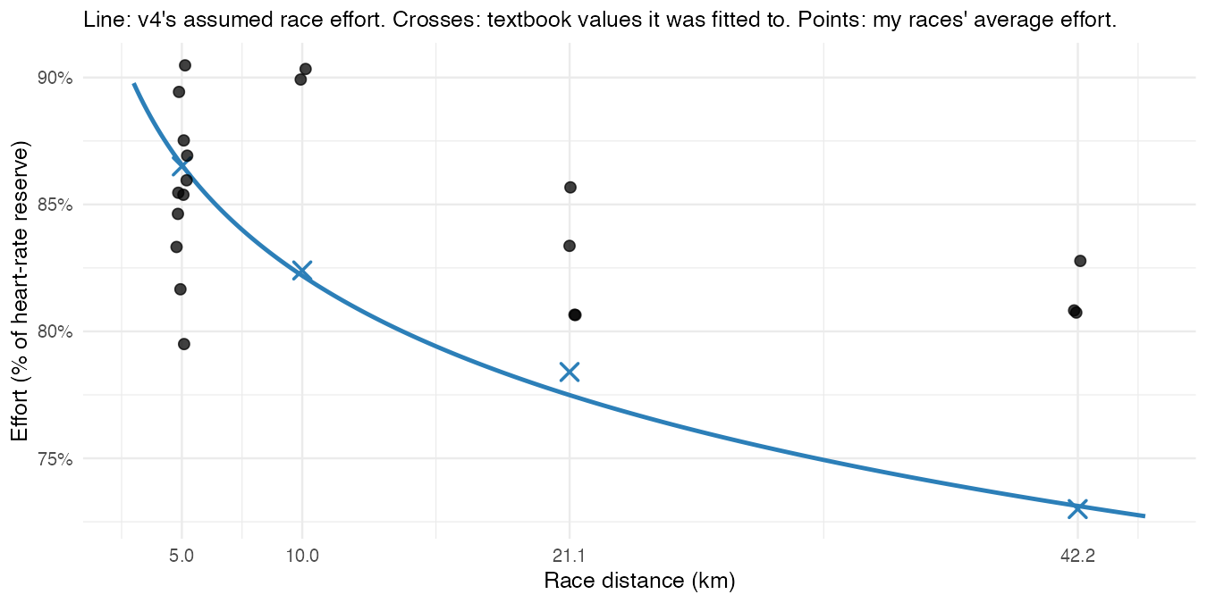
Races were identified as any run with a title containing certain keywords or any run where $e_r \ge 0.85$ (to account for time-trials). This allows race pace predictions for a given distance $D$ to be generated by extrapolating $e^*_r$ from the curve and inputting that value into the likelihood. This curve was obtained by standard tables of % max heart rates at different race distances, converted to % of heart-rate reserve (as $e_r$ is encoded) and is shown below, along with my races overlaid. It makes it abundantly obvious that I’m not quite trained to the same level as the elite athletes who provide those textbook values, as my heart is working far harder at >= half-marathon distance then theirs are!
While this model finally got us closer to being able to predict race times, it was still suffering non-ignorable divergences.
Resuming with Opus 5.5: fixing and frontiering (v5 - v8)
v5: Fixing v4
Because we were still experiencing divergences with v4, I left this analysis for a couple of months thinking I needed to go back to the drawing board. When Opus 5.5 was released it was immediately obvious what a step change this was from previous models, and especially compared to Sonnet 4.6 that I’d been using previously. I decided to let Opus 5.5 at this problem (now running Claude Code) and gave it free reign to change the models as it saw fit. It started a new mode of agentic work, whereby it iterated on differnet models, updating me on sampling progress and when a new model finished.
The first task it set to was trying to fix the flaws with v4, which it saw as:
- Still keeping the $k_F b_F$ identifiability ridge that Sonnet 4.6 completely missed
- Not having a distance term in the pace equation itself, the distance only impacts the pace via the fixed distance curve with effort. The model doesn’t use any information about how my pace changes with distance
- Furthermore, this curve is used twice: both when fitting races, and when predicting. This curve is never compared to my actual data points (see how my marathon used a far higher proportion of my heart rate reserve than the curve allows for).
- Pace is modelled on the natural scale when proportional errors makes more sense and it makes the distance power law linear
- Not accounting for elevation
- Not accounting for increased heart rate when pushing stroller
- Daily mean temperature adds uncertainty that should be captured by the temperature at the start hour
- The previous models predicted the run on day $d$ including the load for that day $L_d$. This allows a hard race (big $L_d$) to explain the run results - a circular argument.
Putting it all together, this was the resultant likelihood:
$$ \log \overline{p}_r \sim \mathcal{N}(\eta_r, \sigma_{[r]}) $$ $$ \eta_r = \mu + b_e(\bar{e} - e_r) + b_1 x_r + b_2 x_r^2 + b_T \Delta T_r + b_E \Delta E_r + b_R \mathbb{1}^{\text{race}}_r + b_{\text{enc}} \mathbb{1}^{\text{enc}}_r - b_F F_d + b_G G_d, $$ $$F_d = a_F F_{d-1} + (1 - a_F) L_{d-1}, \qquad a_F = e^{-1/\tau_F}$$
Which keeps the effort and temperature term ($\Delta T_r = T_r - \bar{T}$) and adds:
- A term accounting for elevation ($\Delta E_r = E_r - \bar{E}$)
- Quadratic terms for the distance $x_r = \log(D_r/10)$ scaled so 10km = 0 and logged to linearize the power curve
- An indicator for whether the run was a race $\mathbb{1}^{\text{race}}_r$ rather than conveying race information through the effort
- An indicator for whether the run was encumbered with a pushchair $\mathbb{1}^{\text{enc}}_r$
- Updates the daily Fitness ($F_d$) and Fatigue ($G_d$) values to use the previous day’s load ($L_{d-1}$)
- Fitness (and fatigue) are reparameterized to replace $k_F$ with $(1-a_F)$, removing the free parameter
These changes finally (well the last change really) removed the sampling problems, with only 1 single divergence being found. This now meant that attention could finally turn to the actual modelled parameters rather than dealing with sampling issues.
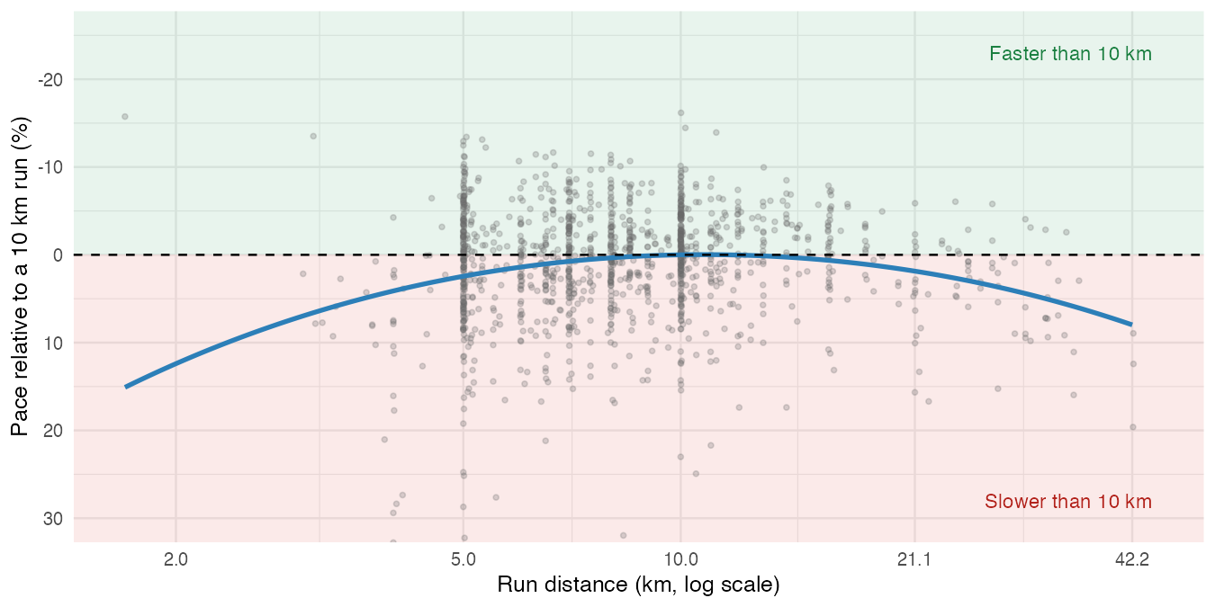
One oddity was the modelled distance effect, plotted below (Figure 2). This shows that the estimated pace is only quicker than 10km pace on distances between 10km and 11.6km, either side of that the predicted pace slows down. This is an artefact of using average pace from the dataset which shows what I did, not what I was capable of. I.e. most of my speedwork sessions would have been in the 10-11.6km range, while the vast majority of my shorter runs would have been easy slow sessions to build up my mileage or recover, rather than going flat out at a 5km race. Therefore the model makes the link that “shorter distance = slower run”.
v6: replacing average pace with best-efforts
Now that Opus 5.5 had proved its worth instantly by fixing the sampling issue and extending v5 with sensible additions, I gave it free reign to iterate with the same objective. I was very impressed by the initiative it took, i.e. it started to evaluate models on multiple evaluation sets: the races, all runs, as well as refitting the models without a held-out set of races. It also provided frequent sampling updates so I could keep an overview of its progress.
The first thing that Opus 5.5 wanted to fix in v6 was the observed data, to replace the average pace used previously, which resulted in the slower race predictions at shorter distances. It wanted to instead search each run for the fastest continuous segment for a range of distances (1km, 5km, 10km, 10mile, half marathon, 30km, marathon + others). These segments are termed best efforts, which straight away increases the number of datapoints from ~1,200 (number of runs) to > 7,000.
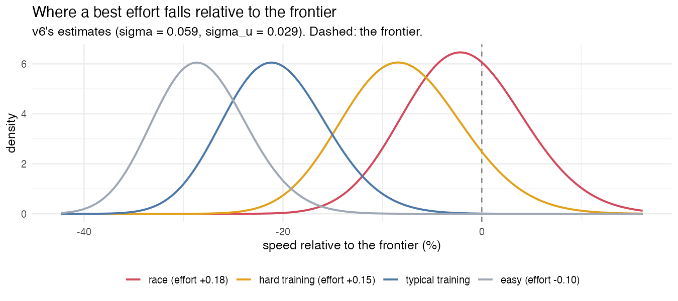
It next changed the form of the likelihood to a “stochastic frontier” - an idea borrowed from econometrics (Aigner et al., 1977) where you model the ideal situation (e.g. perfect race conditions) and then model the “shortfall” that explains the difference from the frontier (not trying hard, it not being a race, etc…).
Each best effort’s speed $v_i$ comprises a frontier $\theta_i$ minus a non-negative shortfall $u_i$:
$$\log v_i = \theta_i - u_i + \varepsilon_i, \qquad \varepsilon_i \sim \mathcal{N}(0, \sigma_v), \qquad u_i \sim \mathcal{N}^+(\mu_i, \sigma_u)$$
The frontier $\theta_i$ is the log of the fastest speed at that distance I could have run on that day, and largely uses the same parameterization as before, incorporating distance, temperature and elevation.
$$\theta_i = \phi(t_i) - \beta_1 x_i - \beta_2 x_i^2 - b_T \Delta T_i - b_E \Delta E_i$$
$\phi(t)$ is the new performance term (aka fitness, but not Banister Fitness $F_d$) and is quantified as the log of the maximum 5km speed I could have ran that day, and the distance terms $x_i$ are now scaled relative to 5km instead of 10km.
The shortfall’s centre $\mu_i$ is smaller the harder I was working, lower in races, and higher when pushing the running stroller:
$$\mu_i = m_0 - m_e (e_i - \bar{e}) - m_f \log(d_i/D_i) - m_R \mathbb{1}^\text{race}_i + m_\text{enc} \mathbb{1}^\text{enc}_i$$
The $\frac{d_i}{D_i}$ adjusts for best efforts that are only a small part of a long run. Say we have 2 best efforts of 5km - one from a 5km run and the whole is taken from a 10 mile training run. In the first scenario this term is 0 (due to log) and doesn’t impact the shortfall. In the second scenario this term contributes $-1.17$ to the shortfall, i.e. increasing the effect of the shortfall on the frontier and hence accounting for why I was wanting running as fast in this effort rather than letting my fitness $\phi$ take a hit.
The other 3 data terms are unchanged (e.g. $e_i$ is the measured data effort as a fraction of heart rate reserve as has been the case since v3). This allows for the separation of “not trying hard” from “less fit” as the effort term now explicitly quantifies the former, leaving $\phi(t)$ for the latter, measured in pace rather than heart-rate. This also allows for simple race prediction times: it’s simply the frontier at the given distance minus a small race shortfall.
Opus then did some magic to integrate out the shortfall (Stevenson, 1980) trying a half-normal before settling on a truncated normal.
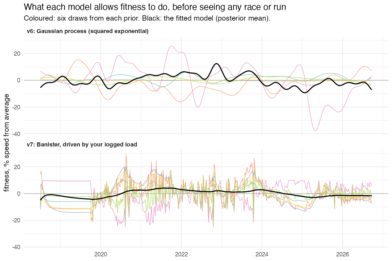
The final change made by Opus was in the dynamics of the fitness term, $\phi(t)$. Fitness has been modelled using the Banister recursive equations since v1, however, Opus wanted to use a more data-driven approach to learn a flexible model from the data rather than be constrained with the Banister equations. In particular it used a Gaussian Process (GP) with a squared-exponential kernel, and then employed some more wizardry to approximate it with “a Hilbert-space basis of 64 sine functions” so it would actually sample (the usual bane of my life when using GPs).
This model sampled very well (assume convergence wasn’t a problem from here on out unless mentioned), and finally we get some race predictions & fitness values that can be evaluated (more on that later).
v7: Banister model instead of GP
Simultaneously to v6, Opus was keen to try the standard Banister model for $\phi(t)$ instead of the GP to identify how much of an impact training load has on fitness, or whether any smooth would work. Apart from $\phi(t)$, v7 was identical to v6. In Figure 4 below we can see the huge difference in flexibility in their priors - the GP can fit any shape whereas the Banister curve is constrained by the load.
While v7 converged eventually, it took a bit of work to get to that point and its held-out refit failed completely. Furthermore the fitness and fatigue decays increased to near the maximum allowed by the prior because only the training load now impacts on $\phi(t)$, leading to very slow moving trends. Therefore, the decision was made to stick with the more flexible GP approach.
v8: fixing the distance curve
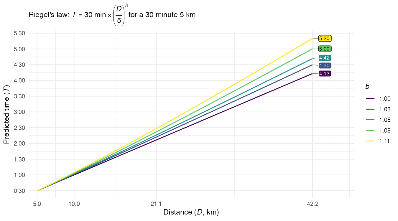
While looking at the v6 posterior predictive diagnostics, Opus noticed a flaw: the distance curve was far too flat. Riegel’s Law is a long-held model relating the time $T_2$ taken to complete a race of distance $D_2$, given that a known race of distance $D_1$ took $T_1$ time as follows
$$ T_2 = T_1 \frac{D_2}{D_1}^{b} $$
where $b$ is an free parameter that typically lies around 1.06. However, after converting $\beta_1$ from v6 into an implied Riegel exponent results in $b=1.03$, far lower than either the textbook value or the implied value from my PBs of 1.11. While this doesn’t sound like much, Figure 5 below shows that given a 30 minute 5km time, this difference in $b$ corresponds to a 50 minute difference in predicted marathon time! This means that v6 is far too optimistic at predicting long distance races.
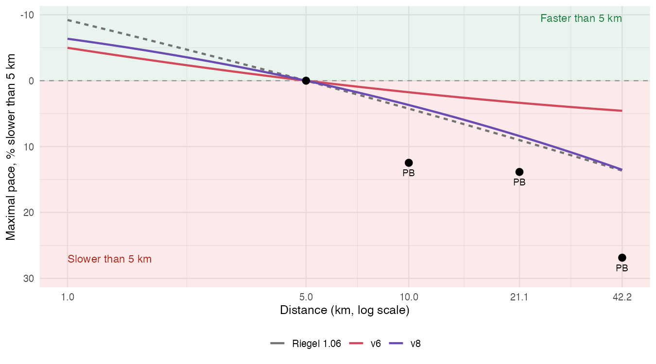
This underestimating of $\beta_1$ is caused by the fact that it is only meaningful for races, i.e. 22 observations, but it is estimated by all >7,000 best efforts. The main modifications for v8 are to the shortfall $\mu_i$ with the intention of only letting the races influence $\beta_1$. The new form is as follows:
$$ \mu_i = \Big( m_0 - m_e(e_i - \bar{e}) - m_f \log(d_i/D_i) + m_{\text{enc}}\mathbb{1}^{\text{enc}}_i + \delta_{d(i)} + \eta_{r(i)} \Big)\big(1 - \mathbb{1}^{\text{race}}_i\big), $$
where:
- $\delta_{d(i)}$ is an offset per distance (remember best efforts have 1 of a possible N values)
- $\mu_i = 0$ for a race
- $d_i$ is the distance of effort $i$ while $D_i$ is the total distance of the run that contained effort $i$
- $\eta_{r(i)}$ is a per run term
Let’s start with the first 2 of these. Because the best efforts are binned into a discrete set of distances, $\delta_{d(i)}$ will counteract $\beta$ as
$$ \log v_i = \phi(t_i) - \beta_1 x_i - \beta_2 x_i^2 - (\ldots + \delta_{d(i)}) + \ldots $$
We can ignore $\beta_2$ as it was negligible and focus on the relationship between $\beta_1 x_i$ and $\delta_{d(i)}$. $x_i$ is the distance of effort $i$, and $\delta_{d(i)}$ is a free parameter specific to this distance. Because of this direct relationship, these two will be unidentifiable through their sum. The model only cares that their sum results in an appropriate value $Z$, it doesn’t matter what the two terms are. This is the exact problem we had with the $k_F b_F$ terms in models v1-v4, but this time it’s intentional. What? Yes, we want $\delta_{d(i)}$ to cancel out the $\beta_1 x_i$ term as $\delta$ only impacts on training data, as the whole shortfall $\mu_i = 0$ for a race effort and hence only races impact the estimation of $\beta_1$. Very clever Opus, well done. Figure 6 shows this has worked well with the curve very neatly following the textbook Riegel $b = 1.06$.
The final shortfall addition from this model is $\eta_{r(i)}$, which is a per-run effect as there is a high amount of correlation between best efforts within the same run (if I ran fast over 3k I’m likely to also run fast over 5k).
In addition to all the shortfall changes, v8 also adds a ‘freshness’ term to the frontier: $\,b_{\text{fresh}} S_{t}$ where $S_t = (A^{7}_t - A^{42}_t)/\text{sd}$. $A^7$ and $A^{42}$ are averages of yesterday’s load with fixed decay times of 7 and 42 days respectively, $\text{sd}$ is just a scaling term. $S_t \gt 0$ when the recent week is heavier than usual, while $S_ \lt 0$ when it’s comparatively light, such as during a taper. $b_{\text{fresh}}$ had an 80% CI that straddled zero, so its impact here is minimal.
Online updates and final tweaks (v9-v12)
v9: Online updating
At this point Opus (which had been working solidly by itself for a few hours) came back up for air, summarized its progress and asked where I’d like to lead it next. I was keen to get an output from this work that I could actually use in practice, rather than just an academic analysis. An obvious outcome is having a model that I can run live with my own fitness tracker, this would mean moving to a model structure that would allow for online Bayesian updating, rather than batch MCMC.
I tasked Opus with keeping the rest of the model as similar as possible, but reframing it in a way that is compatible with online updating and it came up with swapping the squared-exponential GP kernel that we’d been using since v6, for a Matérn-5⁄2. This is defined as follows, for a gap of $s$ days,
$$ \operatorname{Cov}\big(f(t), f(t+s)\big) = \alpha^2 \left(1 + \kappa|s| + \tfrac{\kappa^2 s^2}{3}\right) e^{-\kappa |s|}, \qquad \kappa = \sqrt{5}/\ell, $$
this is exactly the solution of a linear stochastic differential equation (SDE) for $\mathbf{f}(t) = (f, f’, f”)$ (representing fitness and its first two derivatives) (Hartikainen & Särkkä, 2010).
$$ \mathrm{d}\mathbf{f} = \begin{pmatrix} 0 & 1 & 0 \ 0 & 0 & 1 \ -\kappa^3 & -3\kappa^2 & -3\kappa \end{pmatrix} \mathbf{f}\, \mathrm{d}t + \begin{pmatrix} 0 \ 0 \ q \end{pmatrix} \mathrm{d}W_t, \qquad q = \sqrt{16 \kappa^5 / 3}\,\alpha, $$
where $W$ represents Brownian motion (continuous-time noise). The Matérn kernel allows for fitness to respond to intermitten shocks, but is pulled towards a long-term average. It also has the Markov property so that it can be updated online simply in a Kalman Filter.
Whereas previously each model is intended to improve on the previous iteration, for v9 we just wanted to have minimal regression from v8 while retaining the ability to update online. Fortunately, this is exactly what transpired, both when run under MCMC and the Kalman Filter! Hence the Matérn-5⁄2 was used for the rest of the models.
This version was a step-change in terms of the utility that Opus brought - I have never heard of the Matérn kernel family before and implementing it, plus the Kalman Filter implementation using the SDE would have taken me a very long time to get fully working.
v10: fixing race flags
In contrast to v9, the upgrade to v10 was conceptually extremely simple and definitely the sort of thing that AI isn’t needed for, but it yielded a huge improvement in model accuracy. The race flag $\mathbb{1}^{\text{race}}_i$ was previously set to 1 for all best efforts within an identified race, not just the best effort corresponding to the race distance. In other words, the fastest 5km segment run in the middle of a marathon would be have a 0 shortfall and assumed to be the fastest possible 5km I was capable of on that day…
This obvious bug was fixed so that the frontier is correctly estimated, taking 130 race-flagged best efforts down to 19.
While this certainly improved the predicted race times (will follow soon), its impact can also be seen in the implied Riegel $b$ exponent increasing from $\approx 1.06$ in v9 to $\approx 1.10$ in v10 - gettign closer to the implied figure from my PBs of 1.112 (although interestingly moving away from the textbook Riegel $b=1.06$.
v11: calibrating prediction intervals
While the point prediction race time estimates from v10 were very accurate, the prediction intervals were too narrow: only 60% of held out races were within the 80% intervals, indicating a problem with the model spread, not its central tendency. This was addressed by replacing the previous single variance $\sigma_v$ used on all best efforts with a training and race specific one:
$$ \log v_i = \theta_i - u_i + \varepsilon_i, \qquad u_i \sim \mathcal{N}^+(\mu_i, \sigma_u), \qquad \varepsilon_i \sim \mathcal{N}\left(0,\ \sigma_{[i]}\right), $$ $$ \sigma_{[i]} = \begin{cases} \sigma_{\text{race}} & \text{if } \mathbb{1}^{\text{race}}_i = 1 \\ \sigma_v & \text{otherwise} \end{cases} $$
$\sigma_{\text{race}}$ was estimated about 40% larger than $\sigma_v$, which had the desired effect of widening the intervals. Normally you might think that races will have less variation on pace as each race effort should be largely homogenous flat out best efforts, whereas training runs encompasses a huge variety of easy mileage, a variety of speedworks, trail running and so on.
However, that’s because training runs have an additional source of variation: $\eta_r$ is a per-run effect with corresponding variance $\sigma_\eta$, which absorbs the inter-run variance, leaving $\sigma_v$ to account for intra-run variance (i.e. the difference between a 1km and 5km best effort in the same run). Sure enough $\sigma_\eta \gt \sigma_v$. However, races don’t have the $\eta_r$ term as $\mu_i = 0$, and hence there is only 1 source of variation: $\sigma_{\text{race}}$. A more fair comparison on the variance between races and training runs would therefore be:
$$ \sqrt{\sigma_v^2 + \sigma_\eta^2} = \sqrt{0.037^2 + 0.065^2} \approx 0.075 $$ $$ \sigma_{\text{race}} = 0.051 $$
And hence there is more variance in training runs as expected.
v12: bringing training load back
By now we had a model that was producing accurate race estimates, realistic looking fitness curves, and it was all converging well. Opus wanted one final attempt to incorporate the Banister states that had been dropped since v7 to explain why the fitness trend was changing. In models v1-v5 (plus v7) the Banister terms were used to model fitness, before being replced with a single fitness term $\phi_t$ in v6 that is a data-driven estimate by a GP.
In this iteration Opus wanted to model $\phi_t$ as constituting both the deterministic Banister terms $F(t)$ and $G(t)$ as well as the stochastic term $f(t)$ modelled by a GP. In running terms, the Banister terms explain the unchanging response to training load, while the GP absorbs any other source of variation i.e. illness or injury.
$$\phi(t) = \phi_0 + f(t) + b_F F(t) - b_G G(t)$$
Getting this model to sample cleanly was a bit of a challenge as without any constraints $b_F$ and $b_G$ become unidentifiable. In practice this was solved by hardcoding fitness and fatigue to have 2 non-overlapping ranges (1-14 days for fatigue, 28-365 for fitness).
The estimated decay times fit textbook values almost perfectly (fitness was 50 days, fatigue 6 days), with training load accounting for approximately a quarter to a third of the variation in my fitness over the full time frame of my running career. From a predictive perspective, v12 was slightly weaker than some of the previous iterations. However, having the deterministic Banister terms allows for forecasting race predictions into the future for a given training programme (and hence load). While this is a useful functionality, ultimately the biggest test was how well it predicted race times - this is more of my interest than explanatory power, and having training load “only” explain a quarter to a third of fitness suggests that it isn’t that strong an effect.
Results
Finally, the moment of truth: how accurate are these models at predicting my race times? The most unbiased way to assess them is to refit each model omitting some races as a held-out test set and evaluate on those. Evaluating a model on races that were used to estimate the parameters will always lead to an overly optimistic assessment, particularly on a heavily unbalanced dataset like this. This process only leaves 10 held-out races, so we shouldn’t fixate on small differences between scores but instead use these metrics as an additional point of evidence for the bigger picture.
The results are shown in the table below where a positive bias means predictions were too slow, and MAE % is the relative mean absolute error between the predicted race time and the actual. NB: v7 wasn’t run on the held out set due to sampling issues, and v9 wasn’t either because v9 was only mainly assessed on whether it produced the same estimates as v8 but with the new online Matérn kernel. The table highlights how the first model was horriby innacurate, while the subsequent 3 versions to try and improve this instead resulted in poor sampling. v5 stabilized the sampling, but still had a large error on the held out dataset. The next 7 models iteratively improve on this, gradually bring the MAE down with the biggest jump coming from v10’s fix to the race flag. v11 and v12 don’t improve on the point estimates but the intervals are better calibrated and v12 can explain why fitness changed.
v11 is as accurate as any model at 4% mean absolute error, with well-calibrated intervals. v12 is no better on races, but slightly better at predicting ordinary runs it hadn’t seen yet (19 of 23 runs since the fit), and is the only model that can explain why fitness changed.
Sampling | Races (in sample) | Races (held-out) | ||||||
|---|---|---|---|---|---|---|---|---|
| Model | Max R-hat | Divergences | Bias % | MAE % | 80% coverage | Bias % | MAE % | 80% coverage |
| v1 (heart rate at fixed pace) | 1.005 | 6 | -66.5 | 66.5 | 0.20 | – | – | – |
| v2 (latent effort) | 1.310 | 79 | -17.9 | 18.5 | 0.30 | – | – | – |
| v3 (measured effort) | 1.013 | 118 | +9.3 | 9.5 | 1.00 | – | – | – |
| v4 (races, temperature) | 1.006 | 147 | +6.0 | 6.9 | 0.80 | – | – | – |
| v5 (Banister, average pace) | 1.006 | 1 | +1.4 | 7.2 | 0.68 | +7.6 | 8.2 | 0.80 |
| v6 (frontier, GP) | 1.005 | 0 | +0.9 | 6.9 | 0.50 | +3.8 | 6.1 | 0.60 |
| v7 (frontier, Banister) | 1.004 | 0 | +0.8 | 7.4 | 0.73 | – | – | – |
| v8 (races set distance curve) | 1.018 | 0 | +3.2 | 5.6 | 0.45 | +4.4 | 5.9 | 0.40 |
| v9 (Matérn GP) | 1.009 | 0 | +3.0 | 5.3 | 0.45 | – | – | – |
| v10 (race flag fixed) | 1.013 | 0 | -1.2 | 4.9 | 0.55 | 0.0 | 4.0 | 0.60 |
| v11 (race noise) | 1.010 | 0 | -1.4 | 5.2 | 0.68 | -0.1 | 4.0 | 0.90 |
| v12 (+ training load) | 1.009 | 6 | -1.1 | 5.4 | 0.68 | +0.3 | 4.3 | 0.90 |
Figure 7 shows the predicted 5km time over the full 8 years for four representative models: v5, v6, v8, and v11. It firstly shows the huge amount of increased flexiblity from the GP fitness model (v6, v8, v11) over the Banister updates (v5). Secondly, v11 tracks my actual races and time trials far better than the earlier models which are all too pessimistic - when I finally went sub 20min in 2021-2022 the other models didn’t think I was capable of less than 21mins!
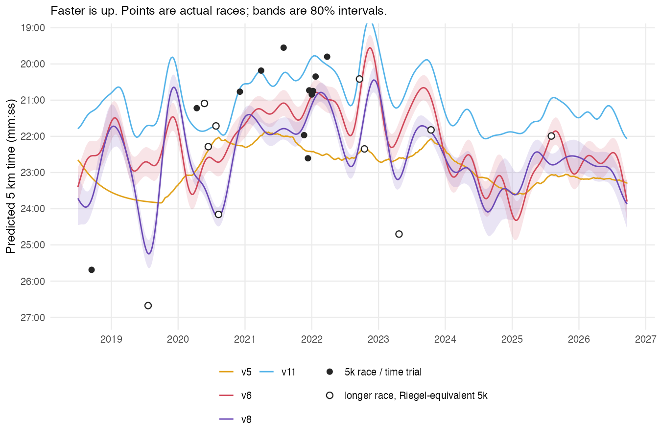
How do the predictions compare to Garmin’s? As of the end of my data (23 September 2026) these estimates are consistently more optimistic than Garmin’s own. This is interesting as I would previously say that Garmin is too optimistic, but here I think it is more realistic and in fact it’s my models that are placing too great an emphasis on my fitness from several years ago.
| Race | v11 | v11 80% interval | Garmin |
|---|---|---|---|
| 5k | 22:19 | 20:44 - 23:56 | 24:06 |
| 10k | 48:22 | 44:49 - 52:01 | 50:56 |
| Half marathon | 1:49:28 | 1:41:23 - 1:57:23 | 1:55:48 |
| Marathon | 3:50:10 | 3:32:23 - 4:08:23 | 4:17:33 |
Conclusions
This experience has been an eye-opener for the value that LLMs can bring to analyses such as this. The LLM was able to help in several ways: suggesting new modelling methodologies, evaluation strategies, writing the Stan syntax, knowledge of fixing sampling issues with Stan tricks, knowledge of various different modelling methods, able to automatically setup watchdogs and monitoring so we caught poorly sampling chains in progress and being able to kill them. I feel that the progress made in 2 days working on this with an LLM far exceeds the work I could have achieved in 2 months solo, unless I’d spent years building up my experience in Stan and this type of tempral modelling with online estimation. Furthermore I could really see the step change from Sonnet 4.6 to Opus 5.5 - it instantly fixed the issues from the 4 attempts that Sonnet had and suggested significant improvements each time. It also provided far more assistance with general tooling, for example Opus 5.5 took complete control of the agentic workflow whereas Sonnet 4.6 was still working in a slower loop where it suggested model changes and I was in charge of implementing and testing them.
In terms of the modelling itself, the main lessons I took home were:
- Data is always the key, not the model Both of the biggest improvements came from changes to how the data was handled: firstly using best efforts with a frontier likelihood and then fixing the race-flag in v10. These changes had far bigger impacts than the more flashy changes such as moving to a GP, or adding the Matérn kernel.
- Training load matters less than is traditionally thought v12 added both training load via the Banister terms alongside a flexible fitness structure, and while the training load was indeed informative, it only accounted for a quarter to a third of the variation in my fitness. Sometimes using neat analytical approximations like this are good enough, but here the data driven approach was far more flexible. I can only imagine what companies like Strava or Garmin can do with millions of different individuals’ data.
- Run more races! The races are key to this model and only having 22 of them is a huge limitation. I should run more races, or at least time-trials, in order to anchor the model periodically - despite how much I hate running flat out. Ideally these time-trials would cover a range of distances but I’m hardly going to run a monthly flat out marathon!
I’ve incorporated these changes into my StravaR dashboard using v11 so that after every data sync my fitness and race predictions get updated. Unfortunately it isn’t possible to make this model publicly available yet as it’s tailored specifically to me, but if you let me know if you’re interested in this functionality I can share with you the Stan model and a script to prepare your data for training.
TODO screenshot
Figure 8: Fitness and predicted race times have been added to the StravaR dashboard and update after each new activity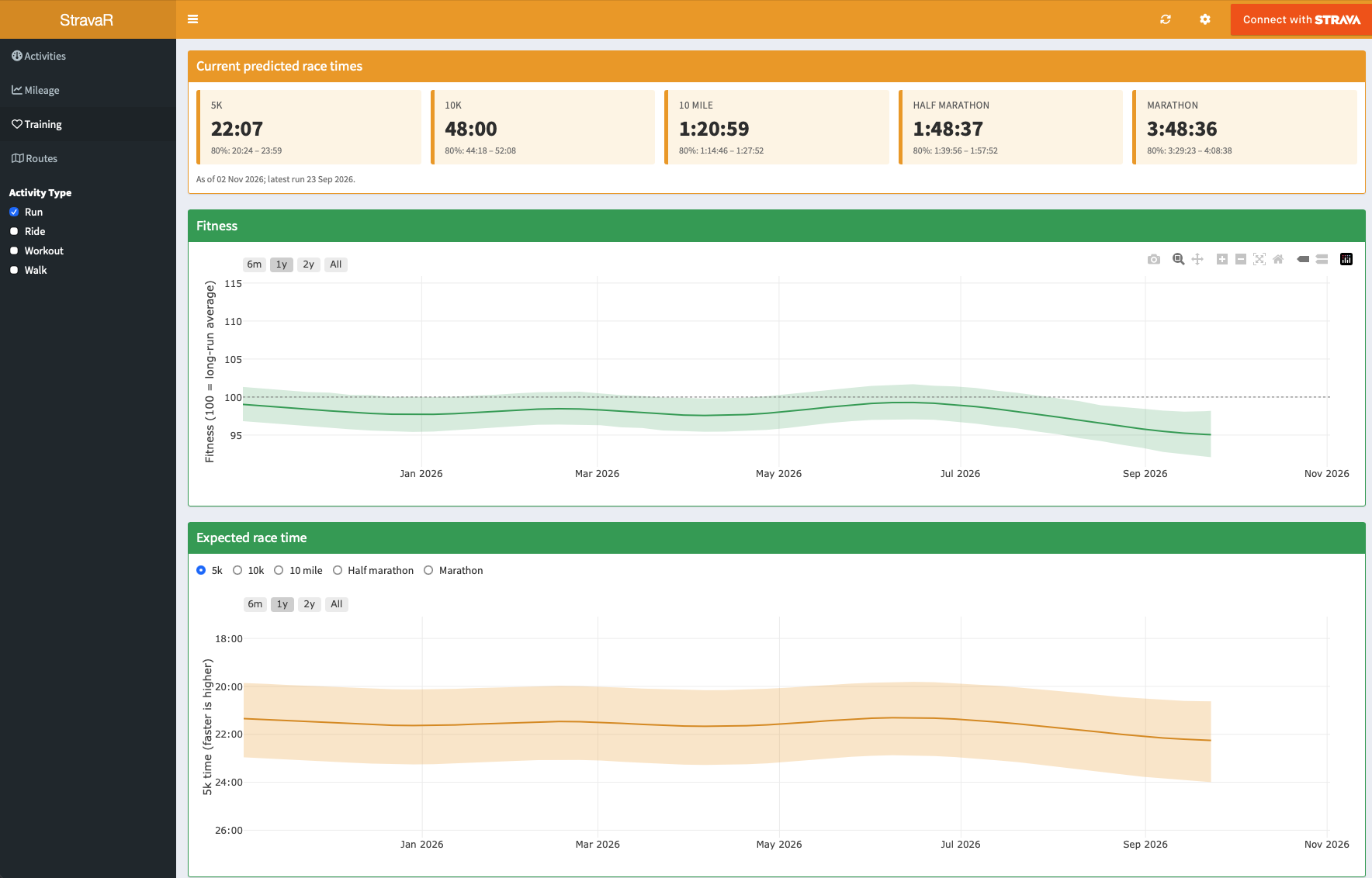
References
- Aigner, D., Lovell, C. A. K. & Schmidt, P. (1977). Formulation and estimation of stochastic frontier production function models. Journal of Econometrics, 6(1), 21-37.
- Banister, E. W., Calvert, T. W., Savage, M. V. & Bach, T. (1975). A systems model of training for athletic performance. Australian Journal of Sports Medicine, 7, 57-61.
- Chopin, N. (2002). A sequential particle filter method for static models. Biometrika, 89(3), 539-552.
- Hartikainen, J. & Särkkä, S. (2010). Kalman filtering and smoothing solutions to temporal Gaussian process regression models. IEEE International Workshop on Machine Learning for Signal Processing, 379-384.
- Riegel, P. S. (1981). Athletic records and human endurance. American Scientist, 69(3), 285-290.
- Stevenson, R. E. (1980). Likelihood functions for generalized stochastic frontier estimation. Journal of Econometrics, 13(1), 57-66.