Introduction
And so finally we come to the end of this comparison of four different modelling strategies for predicting football matches: hierarchical Bayesian regression models, a traditional Elo rating system, an optimised Elo system using Evolutionary Algorithms (EAs), and online Bayesian models using Particle Filters. I’ll skip most of the code so we can jump straight to the results, but it’s all available by clicking on the folds in the following section.
Preparing the environment
Loading R packages
library(tidyverse)
library(data.table)
library(e1071)
library(cmdstanr)
library(parallel)
library(ggrepel)
library(rethinking)
library(plotly)
library(knitr)
library(kableExtra)
options(knitr.table.html.attr = "quarto-disable-processing=true")
options(cmdstanr_draws_format = "draws_matrix")
Prepare reticulate with Python dependencies
Sys.setenv("RETICULATE_USE_MANAGED_VENV"="yes")
library(reticulate)
py_require(
    c(
        "particles==0.4",
        "pandas==2.3.3",
        "numpy",
        "scipy",
        "matplotlib",
        "seaborn"
    ),
    python_version = ">=3.13"
)
Load Python dependencies
import particles
import pandas as pd
from scipy.stats import norm, poisson
import particles.state_space_models as ssm
import particles.distributions as dists
from particles.collectors import Moments
import pickle
import numpy as np
Preparing dataset
df <- readRDS("data/df_wld.rds")
leagues <- levels(factor(df$league))
leagues <- setNames(leagues, leagues)
training_teams <- df |>
    filter(dset == 'training') |>
    distinct(home) |>
    pull(home)

df <- df |> mutate(matchid = row_number())

# Add number match of season for as some models use it
home_games <- df |>
    distinct(matchid, season, date, team=home, league)
away_games <- df |>
    distinct(matchid, season, date, team=away, league)
matches_in_season <- home_games |>
    rbind(away_games) |>
    arrange(league, season, team, date) |>
    group_by(league, season, team) |>
    mutate(match_of_season = row_number()) |>
    ungroup() |>
    select(matchid, team, match_of_season)
team_ids <- read_csv("data/team_ids.csv")
df <- df |>
    inner_join(
        matches_in_season |>
            rename(
                home=team,
                home_match_of_season=match_of_season
            ),
       by=c("matchid", "home")
    ) |>
    inner_join(
        matches_in_season |>
            rename(
                away=team,
                away_match_of_season=match_of_season
            ),
        by=c("matchid", "away")
    ) |>
    mutate(
        result_int = as.integer(
            factor(
                result,
                levels=c("away", "draw", "home")
            )
        )
    ) |>
    inner_join(
        team_ids |> select(home, home_id=team_id), by="home"
    ) |>
    inner_join(
        team_ids |> select(away=home, away_id=team_id), by="away"
    )
Convert to data.table for speed
setDT(df)
setorderv(df, "date")
Create columns to hold model predictions
models <- c(
    'naive_bayes',
    'hierarchical_ordinal',
    'hierarchical_poisson',
    'elo_ordinal',
    'elo_poisson',
    'elo_nn',
    'particle_poisson',
    'particle_ordinal'
)
preds <- lapply(setNames(models, models), function(x) NULL)
for (m in models) {
    for (o in c('away', 'draw', 'home')) {
        col <- sprintf("pred_probs_%s_%s", m, o)
        df[, (col) := NA_real_ ]
        if (grepl('poisson', m)) {
            pois_col <- sprintf("pred_goals_%s_%s", m, o)
            df[, (pois_col) := NA_integer_ ]
        }
    }
}
Load Naive Bayes model
mod_nb <- readRDS("models/naive_bayes.rds")
predict_nb <- function(row) {
    predict(mod_nb, row, type='raw')
}
Load hierarchical ordinal logistic regression model
inv_logit <- function(x) {
    exp(x) / (1 + exp(x))
}

draw_ordinal_logistic <- function(cutpoints, lps) {
    n_outcomes <- dim(cutpoints)[2] + 1
    cum_probs <- inv_logit(apply(cutpoints, 2, function(x) lps - x))
    probs <- matrix(0, nrow=nrow(cum_probs), ncol=n_outcomes)
    probs[, 1] <- 1- cum_probs[, 1]
    probs[, n_outcomes] <- cum_probs[, n_outcomes-1]
    for (i in seq(2, n_outcomes-1)) {
        probs[, i] <- cum_probs[, i-1] - cum_probs[, i]
    }
    pred_outcomes <- apply(probs, 1, function(x) rcategorical(1, x))
    preds <- as.numeric(table(pred_outcomes) / nrow(probs))
    tibble(away_prob=preds[1], draw_prob=preds[2], home_prob=preds[3])
}

fit_ord_log_3 <- readRDS("models/hierarchical_ordinal_league_winloss.rds")
predict_ordinal_3 <- function(home, away, league=NULL, home_win=0, home_loss=0, away_win=0, away_loss=0, ...) {
    # Returns probabilities in away/draw/home
    home_id <- match(home, training_teams)
    away_id <- match(away, training_teams)
    league_id <- match(league, leagues)

    if (!is.na(home_id)) {
        skills_home <- fit_ord_log_3$draws(sprintf("skill[%d]", home_id))
    } else {
        # Draw random team
        skill_params <- fit_ord_log_3$draws(c("skill_mu", "skill_sigma"))
        skills_home <- rnorm(nrow(skill_params), skill_params[, 1], skill_params[, 2])
    }

    if (!is.na(away_id)) {
        skills_away <- fit_ord_log_3$draws(sprintf("skill[%d]", away_id))
    } else {
        # Draw random team
        skill_params <- fit_ord_log_3$draws(c("skill_mu", "skill_sigma"))
        skills_away <- rnorm(nrow(skill_params), skill_params[, 1], skill_params[, 2])
    }

    beta <- fit_ord_log_3$draws("beta")
    lps <- (skills_home - skills_away) + beta %*% c(home_win, home_loss, away_win, away_loss)
    # Need to draw cutpoints specifically for this league
    cutpoint_cols <- sprintf("cutpoints[%d,%d]", league_id, 1:2)
    cutpoints <- fit_ord_log_3$draws(cutpoint_cols)
    draw_ordinal_logistic(cutpoints, lps)
}
Load hierarchical Poisson model
fit_pois_4 <- readRDS("models/hierarchical_poisson_2score_league_correlated.rds")
predict_poisson_4 <- function(home, away, league=NULL, home_win=0, home_loss=0, away_win=0, away_loss=0, ...) {
    home_id <- match(home, training_teams)
    away_id <- match(away, training_teams)
    league_id <- match(league, leagues)

    if (!is.na(home_id)) {
        skill_attack_home <- fit_pois_4$draws(sprintf("skill_attack[%d]", home_id))
        skill_defend_home <- fit_pois_4$draws(sprintf("skill_defend[%d]", home_id))
    } else {
        # Draw random team
        skill_params <- fit_pois_4$draws(c("skill_mu", "skill_sigma"))
        skill_overall <- rnorm(nrow(skill_params), skill_params[, 1], skill_params[, 2])
        # Draw attack and defend skills
        skill_attack_home <- rnorm(length(skill_overall), skill_overall, 2.5)
        skill_defend_home <- rnorm(length(skill_overall), skill_overall, 2.5)
    }

    if (!is.na(away_id)) {
        skill_attack_away <- fit_pois_4$draws(sprintf("skill_attack[%d]", away_id))
        skill_defend_away <- fit_pois_4$draws(sprintf("skill_defend[%d]", away_id))
    } else {
        # Draw random team
        skill_params <- fit_pois_4$draws(c("skill_mu", "skill_sigma"))
        skill_overall <- rnorm(nrow(skill_params), skill_params[, 1], skill_params[, 2])
        # Draw attack and defend skills
        skill_attack_away <- rnorm(length(skill_overall), skill_overall, 2.5)
        skill_defend_away <- rnorm(length(skill_overall), skill_overall, 2.5)
    }

    intercept_cols <- sprintf(c("alpha_home[%d]", "alpha_away[%d]"), league_id)
    intercepts <- fit_pois_4$draws(intercept_cols)

    goals_home <- rpois(nrow(intercepts), exp(intercepts[, 1] + skill_attack_home - skill_defend_away))
    goals_away <- rpois(nrow(intercepts), exp(intercepts[, 2] + skill_attack_away - skill_defend_home))
    tibble(
        away_prob=mean(goals_away > goals_home),
        draw_prob=mean(goals_away == goals_home),
        home_prob=mean(goals_away < goals_home),
        goals_away = floor(median(goals_away)),
        goals_home = floor(median(goals_home))
    )
}
Elo rating update functions
G_func <- function(MOV, dr=0) {
    if (MOV <= 1) 1 else  log2(MOV * 1.7) * (2 / (2 + 0.001 * dr))
}

ratings_update_elo <- function(home_score, away_score, home_elo, away_elo, league, result) {

    K <- 20
    HA <- list(
        "premiership"=64,
        "laliga"=68,
        "bundesliga1"=56,
        "seriea"=66
    )[[league]]

    # Calculate E
    dr_home = (home_elo + HA) - away_elo
    E_home = 1 / (1 + 10 ** (-dr_home / 400.0))
    E_away = 1 - E_home

    # Calculate G
    MOV = abs(home_score - away_score)
    G = G_func(MOV, dr_home)
    O = list(
        'away'= 0,
        'draw'= 0.5,
        'home'= 1
    )[[result]]


    # Calculate updates
    update_home = K * G * (O - E_home)
    update_away = K * G * ((1 - O) - E_away)

    # Update elos
    new_home = round(home_elo + update_home)
    new_away = round(away_elo + update_away)

    c(new_home, new_away)
}
Load Elo ordinal logistic prediction model
mod_elo_ordinal <- readRDS("~/Dropbox/computing/dev/Predictaball/predictors/football/elo/elomodel_final.rds")
predict_elo_ordinal <- function(league, elo_diff) {
    coefs <- mod_elo_ordinal$coefs

    logistic <- function(x) 1 / (1 + exp(-x))

    league_num <- which(mod_elo_ordinal$leagues == league)
    alpha_1_col <- paste0("alpha[", league_num, ",1]")
    alpha_2_col <- paste0("alpha[", league_num, ",2]")

    # Calculate lp
    elo_scale <- (elo_diff - mod_elo_ordinal$elodiff_center) / mod_elo_ordinal$elodiff_scale
    lp <- coefs[, "beta"] * elo_scale

    # Calculate Q values
    Q <- matrix(NA, nrow=15000, ncol=2) # Should be 15K when final
    p <- matrix(NA, nrow=15000, ncol=3) # Should be 15K when final
    Q[, 1] <- logistic(coefs[, alpha_1_col] - lp)
    Q[, 2] <- logistic(coefs[, alpha_2_col] - lp)

    p[, 1] <- Q[, 1]
    p[, 2] <- Q[, 2] - Q[, 1]
    p[, 3] <- 1 - Q[, 2]

    pred_outcomes <- apply(p, 1, function(x) rcategorical(1, x))
    preds <- as.numeric(table(pred_outcomes) / nrow(p))
    tibble(away_prob=preds[1], draw_prob=preds[2], home_prob=preds[3])
}
Load Elo poisson prediction model
mod_elo_poisson <- readRDS("~/Dropbox/computing/dev/Predictaball/predictors/football/elo/coefs_FINAL_elo_goals_20180804.rds")
predict_elo_poisson <- function(league, elo_diff) {
    coefs <- mod_elo_poisson$coefs

    league_num <- which(mod_elo_poisson$leagues == league)
    alpha_home_col <- paste0("alpha_home[", league_num, "]")
    alpha_away_col <- paste0("alpha_away[", league_num, "]")

    # Calculate lps
    elo_scale <- (elo_diff - mod_elo_poisson$elodiff_center) / mod_elo_poisson$elodiff_scale
    mu_home <- coefs[, alpha_home_col] + coefs[, "beta_home"] * elo_scale
    mu_away <- coefs[, alpha_away_col] + coefs[, "beta_away"] * elo_scale

    # Calculate predicted goals
    goals_home <- rpois(length(mu_home), exp(mu_home))
    goals_away <- rpois(length(mu_away), exp(mu_away))
    tibble(
        away_prob=mean(goals_away > goals_home),
        draw_prob=mean(goals_away == goals_home),
        home_prob=mean(goals_away < goals_home),
        goals_away = floor(median(goals_away)),
        goals_home = floor(median(goals_home))
    )
}
Load evolved Elo rating update and prediction models
predict_rposa <- readRDS("/home/stuart/Dropbox/computing/dev/Predictaball/predictors/football/rposa/nn_match_prediction_20190807.rds")
rposa_rating_func <- readRDS("/home/stuart/Dropbox/computing/dev/Predictaball/predictors/football/rposa/nn_rating_update_20190807.rds")
rating_update_rposa <- function(home_score, away_score, home_elo, away_elo, league, result, away_prob, draw_prob, home_prob) {
    probs <- c(away_prob, draw_prob, home_prob)
    mov <- abs(home_score - away_score)
    update_home <- rposa_rating_func(probs, mov, league, result)
    update_away = -update_home
    c(home_elo + update_home, away_elo + update_away)
}
Load ordinal logistic regression Particle Filter
def get_team_PX(xp, t, team_id, var):
    if HOME_ID == team_id:
        mult = 2 if HOME_SEASON_MATCHES < 5 else 1
        return dists.Normal(loc=xp, scale=mult * var)
    elif AWAY_ID == team_id:
        mult = 2 if AWAY_SEASON_MATCHES < 5 else 1
        return dists.Normal(loc=xp, scale=mult * var)
    else:
        return dists.Dirac(loc=xp)

def inv_logit(x):
    return 1 / (1 + np.exp(-x))

def dcat_log(prob, outcome):
    return np.log(prob)*outcome + np.log(1-prob)*(1-outcome)

def get_probabilities(phi, intercepts):
    # X is scalar
    # Phi is N_particles
    # intercepts is 3
    # Form multi-D intercepts
    N_particles = phi.size
    n_outcomes = intercepts.size + 1
    intercepts = np.repeat(np.array([intercepts]), N_particles, axis=0)
    q = inv_logit(intercepts - phi.reshape((N_particles, 1)))
    probs = np.zeros((N_particles, n_outcomes))
    probs[:, 0] = q[:, 0]
    for i in range(1, n_outcomes-1):
        probs[:, i] = q[:, i] - q[:, i-1]
    probs[:, n_outcomes-1] = 1-q[:, n_outcomes-2]
    return probs


class OrdLogit(particles.distributions.ProbDist):
    def __init__(self, phi, kappa1, kappa2):
        self.phi = phi
        self.kappa = np.array([kappa1, kappa2])

    def logpdf(self, x):
        probs = get_probabilities(self.phi, self.kappa)
        return dcat_log(probs[:, x[0]-1], 1)  # NB: need to explicitly cast x as scalar

    def rvs(self, size=None):
        probs = get_probabilities(self.phi, self.kappa)
        cumprobs = np.cumsum(probs, axis=1)
        thresh = np.random.uniform(size=probs.shape[0])
        draws = np.argmax(cumprobs.T > thresh, axis=0) + 1  # + 1 to convert into 1-index
        return draws

    def ppf(self, u):
        print(f"IN PPF")
        pass
    pass

class Ordinal1(ssm.StateSpaceModel):
    def PX0(self):  # Distribution of X_0
        return dists.IndepProd(
            *[dists.Dirac(loc=0) for _ in range(N_TEAMS)]
        )
    def PX(self, t, xp):  # Distribution of X_t given X_{t-1}
        # update X so either have random walk or Dirac
        distributions = [get_team_PX(xp[:, i], t, i, self.skill_walk_variance) for i in range(N_TEAMS)]
        return dists.IndepProd(*distributions)

    def PY(self, t, xp, x):  # Distribution of Y_t given X_t (and X_{t-1})
        lp = x[:, HOME_ID] - x[:, AWAY_ID]
        return OrdLogit(phi=lp, kappa1=self.kappa1, kappa2=self.kappa2)

# Loads the parameters optimised by PMMH
def load_league_params_ordinal(league):
    with open(f"models/ordinal_pmmh_{league}.pkl", 'rb') as infile:
        res = pickle.load(infile)
    params_names = ['skill_walk_variance', 'kappa1', 'kappa2']
    return {p: np.median(res.chain.theta[p][500:]) for p in params_names}

# Predicts match outcome
def predict_match_ordinal(home_id, away_id):
    lp = filter_ordinal.X[:, int(home_id)] - filter_ordinal.X[:, int(away_id)]
    ord_dist = OrdLogit(
        phi=lp,
        kappa1=filter_ordinal.fk.ssm.kappa1,
        kappa2=filter_ordinal.fk.ssm.kappa2
    )
    preds = ord_dist.rvs()
    return pd.DataFrame({
        'away_prob': np.mean(preds == 1),
        'draw_prob': np.mean(preds == 2),
        'home_prob': np.mean(preds == 3)
    }, index=[0])
Load poisson Particle Filter
class PoissonFilter(ssm.StateSpaceModel):
    def PX0(self):  # Distribution of X_0
        return dists.IndepProd(
            *[dists.Dirac(loc=0) for _ in range(N_TEAMS)]
        )
    def PX(self, t, xp):  # Distribution of X_t given X_{t-1}
        # update X so either have random walk or Dirac
        distributions = [get_team_PX(xp[:, i], t, i, self.skill_walk_variance) for i in range(N_TEAMS)]
        return dists.IndepProd(*distributions)

    def PY(self, t, xp, x):  # Distribution of Y_t given X_t (and X_{t-1})
        lp_home = np.exp(self.home_intercept + x[:, HOME_ID] - x[:, AWAY_ID])
        lp_away = np.exp(self.away_intercept + x[:, AWAY_ID] - x[:, HOME_ID])
        return dists.IndepProd(
            dists.Poisson(rate=lp_home),
            dists.Poisson(rate=lp_away)
        )

# Loads parameters optimized by PMMH
def load_league_params_poisson(league):
    with open(f"models/pmmh_{league}.pkl", 'rb') as infile:
        res = pickle.load(infile)
    params_names = ['skill_walk_variance', 'home_intercept', 'away_intercept']
    return {p: np.median(res.chain.theta[p][500:]) for p in params_names}

# Predicts number of goals scored
def predict_match_poisson(home_id, away_id):
    lp_home = np.exp(filter_poisson.fk.ssm.home_intercept + filter_poisson.X[:, int(home_id)] - filter_poisson.X[:, int(away_id)])
    lp_away = np.exp(filter_poisson.fk.ssm.away_intercept + filter_poisson.X[:, int(away_id)] - filter_poisson.X[:, int(home_id)])
    pred_home = poisson.rvs(lp_home)
    pred_away = poisson.rvs(lp_away)
    return pd.DataFrame({
        'away_prob': np.mean(pred_home < pred_away),
        'draw_prob': np.mean(pred_home == pred_away),
        'home_prob': np.mean(pred_home > pred_away),
        'away_goals': np.floor(np.median(pred_away)),
        'home_goals': np.floor(np.median(pred_home))
    }, index=[0])
Functions to instantiate particle filters
def new_season(poisson_X=None, ordinal_X=None, poisson_Xp=None, ordinal_Xp=None):
    if poisson_X is not None:
        filter_poisson.X = poisson_X
    if ordinal_X is not None:
        filter_ordinal.X = ordinal_X
    if poisson_Xp is not None:
        filter_poisson.Xp = poisson_Xp
    if ordinal_Xp is not None:
        filter_ordinal.Xp = ordinal_Xp

def setup_models(league, N_teams):
    global filter_ordinal
    global filter_poisson
    global N_TEAMS
    N_TEAMS = int(N_teams)

    # Poisson model
    # Load PMMH parameters
    pois_params = load_league_params_poisson(league)
    filter_poisson = particles.SMC(
        fk=ssm.Bootstrap(
            ssm=PoissonFilter(
                **pois_params
            ),
            data=np.array([0])
        ),
        N=1000,
        collect=[Moments()]
    )

    # Ordinal model
    ord_params = load_league_params_ordinal(league)
    # swap kappas
    kappa1 = min(ord_params['kappa1'], ord_params['kappa2'])
    kappa2 = max(ord_params['kappa1'], ord_params['kappa2'])
    ord_params['kappa1'] = kappa1
    ord_params['kappa2'] = kappa2

    filter_ordinal = particles.SMC(
        fk=ssm.Bootstrap(
            ssm=Ordinal1(
                **ord_params
            ),
            data=np.array([0])
        ),
        N=1000,
        collect=[Moments()]
    )
Helper functions for particle filters
# Wrapper function that updates both filters with a new match result
# Not needed, but useful to reduce the amount of R <-> Python calls
# Updates each filter separately and returns the updated rating of each team
def update_filters(
    home_id,
    away_id,
    home_season_matches,
    away_season_matches,
    home_score,
    away_score,
    result,
    i
    ):
    global HOME_ID
    global AWAY_ID
    global HOME_SEASON_MATCHES
    global AWAY_SEASON_MATCHES
    HOME_ID = int(home_id)
    AWAY_ID = int(away_id)
    HOME_SEASON_MATCHES = int(home_season_matches)
    AWAY_SEASON_MATCHES = int(away_season_matches)
    update_poisson(int(home_score), int(away_score), int(i))
    update_ordinal(int(result), int(i))
    return [
        get_elo_ordinal(int(home_id)),
        get_elo_ordinal(int(away_id)),
        get_elo_poisson(int(home_id)),
        get_elo_poisson(int(away_id)),

    ]

# Updates the Ordinal particle filter with a new match result
def update_ordinal(result, i):
    # NB: i is 0-indexed
    data_point = np.array([[result]])
    if i >= 1:
        padding = np.repeat(np.array([[0]]), i, axis=0)
        data_point = np.concatenate((padding, data_point))
    filter_ordinal.fk.data = data_point
    next(filter_ordinal)

# Updates the Poisson particle filter with a new match result
def update_poisson(home_score, away_score, i):
    # NB: i is 0-indexed
    data_point = np.array([[home_score, away_score]])
    if i >= 1:
        padding = np.repeat(np.array([[0, 0]]), i, axis=0)
        data_point = np.concatenate((padding, data_point))
    filter_poisson.fk.data = data_point
    next(filter_poisson)

# Gets the rating of a given team from the Ordinal particle filter
def get_elo_ordinal(team_id):
    return filter_ordinal.X[:, team_id].mean()

# Gets the rating of a given team from the Poisson particle filter
def get_elo_poisson(team_id):
    return filter_poisson.X[:, team_id].mean()

# Retrieves the rating states from both filters
def get_end_of_season_states():
    return [
        [
            filter_poisson.X,
            filter_poisson.Xp,
        ],
        [
            filter_ordinal.X,
            filter_ordinal.Xp
        ]
    ]
Main function
AVG_ELO <- 2000
calculate_elo <- function(in_league) {
    ldata <- df[ league == in_league ]
    ldata[, home_id_season := NA ]
    ldata[, away_id_season := NA ]
    start_date <- ldata[, min(date)] - days(10)

    # Identify seasons
    first_season <- TRUE
    seasons <- sort(ldata[, unique(season)])
    last_seasons_teams <- character()

    # Setup particle filter (or just have 1 big one?! would require refactoring to
    # use 1 big dataset as it relies upon having access to the global variable
    # containing all the matches from all the seasons)
    N_teams <- length(ldata[ season == seasons[1], unique(home)])
    py$setup_models(in_league, N_teams)
    match_count <- 0

    # Loop through seasons
    for (j in 1:length(seasons)) {
        cat(sprintf("Season %d/%d (%0.1f%%)\n", j, length(seasons), j/length(seasons)*100))
        this_seasons_teams <- ldata[ season == seasons[j], unique(home) ]
        seas_start_date <- ldata[ season == seasons[j], min(date)] - days(7)

        if (first_season) {
            # Set starting elo to average
            elo_history <- setNames(lapply(this_seasons_teams, function(t)
                data.frame(date = start_date, elo = AVG_ELO)),
                this_seasons_teams)
            elo_nn_history <- setNames(lapply(this_seasons_teams, function(t)
                data.frame(date = start_date, elo = AVG_ELO)),
                this_seasons_teams)
            elo_particle_ordinal_history <- setNames(lapply(this_seasons_teams, function(t)
                data.frame(date = start_date, elo = 0)),
                this_seasons_teams)
            elo_particle_poisson_history <- setNames(lapply(this_seasons_teams, function(t)
                data.frame(date = start_date, elo = 0)),
                this_seasons_teams)
            elo_curr <- setNames(lapply(this_seasons_teams, function(t) AVG_ELO), this_seasons_teams)
            elo_nn_curr <- setNames(lapply(this_seasons_teams, function(t) AVG_ELO), this_seasons_teams)
            elo_particle_poisson_curr <- setNames(lapply(this_seasons_teams, function(t) 0), this_seasons_teams)
            elo_particle_ordinal_curr <- setNames(lapply(this_seasons_teams, function(t) 0), this_seasons_teams)
        }


        # Handle relegation/promotion
        if (!first_season) {
            relegated <- setdiff(last_seasons_teams, this_seasons_teams)
            promoted <- setdiff(this_seasons_teams, last_seasons_teams)
            if (length(relegated) != length(promoted))
                stop("Error: Have unbalanced number of promoted and relegated teams: ",
                     paste(relegated),
                     " are relegated and promoted are ",
                     paste(promoted))
            # Assign promoted teams the average elo of relegated teams
            for (t in promoted) {
                elo_curr[[t]] <- mean(unlist(elo_curr)[relegated])
                elo_nn_curr[[t]] <- mean(unlist(elo_nn_curr)[relegated])
            }

            # Reset everyone's score to 0.8x
            for (team in this_seasons_teams) {
                new_elo <- 0.8 * elo_curr[[team]] + 0.2 * AVG_ELO

                elo_history[[team]] <- rbind(
                    elo_history[[team]],
                    data.frame(date = seas_start_date, elo = new_elo)
                )
                elo_curr[[team]] <- new_elo

                new_elo_nn <- 0.8 * elo_nn_curr[[team]] + 0.2 * AVG_ELO

                elo_nn_history[[team]] <- rbind(
                    elo_nn_history[[team]],
                    data.frame(date = seas_start_date, elo = new_elo_nn)
                )
                elo_nn_curr[[team]] <- new_elo_nn
            }
        }

        # Particle filter setup
        if (!first_season) {
            # Resume the particle filter states from the last season
            new_states <- lapply(prev_states, identity) # Creates a copy
            id_map <- ldata[season == seasons[j]] |>
                mutate(new_id = as.integer(factor(home, levels=this_seasons_teams))-1) |>
                filter(home %in% this_seasons_teams) |>
                distinct(home, old_id=home_id_season, new_id)
            unused_ids <- setdiff(id_map$new_id, id_map$old_id)
            relegated_elo_ord <- mean(unlist(elo_particle_ordinal_curr)[relegated])
            relegated_elo_pois <- mean(unlist(elo_particle_poisson_curr)[relegated])
            for (k in 1:nrow(id_map)) {
                # Set team's state in new location to old
                new <- id_map$new_id[k] + 1  # Convert to 1-index for indexing matrix
                old <- id_map$old_id[k] + 1
                # If team wasn't in league last season, set states to average relegated
                if (is.na(old)) {
                    # New states is [Pois, Ord], then an inner list of [X, Xp]
                    new_states[[1]][[1]][, new] <- relegated_elo_pois
                    new_states[[1]][[2]][, new] <- relegated_elo_pois
                    new_states[[2]][[1]][, new] <- relegated_elo_ord
                    new_states[[2]][[2]][, new] <- relegated_elo_ord
                } else {
                    new_states[[1]][[1]][, new] <- prev_states[[1]][[1]][, old]
                    new_states[[1]][[2]][, new] <- prev_states[[1]][[2]][, old]
                    new_states[[2]][[1]][, new] <- prev_states[[2]][[1]][, old]
                    new_states[[2]][[2]][, new] <- prev_states[[2]][[2]][, old]
                }
            }
        } else {
            new_states <- list(NULL, NULL)
        }
        # Create teamids for this seasons teams
        ldata[, home_id_season := as.integer(factor(home, levels=this_seasons_teams))-1]
        ldata[, away_id_season := as.integer(factor(away, levels=this_seasons_teams))-1]
        seas_data <- ldata[season == seasons[j]]
        py$new_season(new_states[[1]][[1]], new_states[[2]][[1]], new_states[[1]][[2]], new_states[[2]][[2]])

        # Loop through each game (ordered)
        for (i in seq(nrow(seas_data))) {
            cat(sprintf("Game %d\n", i))
            match_count <- match_count + 1 # Global match counter for particle filter
            game <- seas_data[i, ]
            home_elo <- elo_curr[[game$home]]
            away_elo <- elo_curr[[game$away]]
            home_elo_nn <- elo_nn_curr[[game$home]]
            away_elo_nn <- elo_nn_curr[[game$away]]

            if (is.na(game$result)) next

            # Predict match outcomes and goals
            if (sum(game$home_win, game$home_draw, game$home_loss, game$away_win, game$away_draw, game$away_loss) == 10) {
                preds$naive_bayes <- predict_nb(game)
            } else {
                preds$naive_bayes <- rep(NA, 3)
            }

            preds$hierarchical_ordinal <- predict_ordinal_3(
                game$home,
                game$away,
                game$league,
                game$home_win,
                game$home_loss,
                game$away_win,
                game$away_loss
            )
            preds$hierarchical_poisson <- predict_poisson_4(
                game$home,
                game$away,
                game$league,
                game$home_win,
                game$home_loss,
                game$away_win,
                game$away_loss
            )
            preds$elo_ordinal <- predict_elo_ordinal(game$league, home_elo - away_elo)
            preds$elo_poisson <- predict_elo_poisson(game$league, home_elo - away_elo)
            preds$elo_nn <- predict_rposa(game$league, home_elo_nn - away_elo_nn)

            # Can only run filter predictions after first update
            if (match_count > 1) {
                preds$particle_poisson <- py$predict_match_poisson(game$home_id_season, game$away_id_season)
                preds$particle_ordinal <- py$predict_match_ordinal(game$home_id_season, game$away_id_season)
            } else {
                preds$particle_poisson <- rep(NA_real_, 5)
                preds$particle_ordinal <- rep(NA_real_, 3)
            }

            # Save predictions
            for (mod in names(preds)) {
                for (k in 1:3) {
                    col <- sprintf("pred_probs_%s_%s", mod, c('away', 'draw', 'home')[k])
                    ldata[ matchid == game$matchid, (col) := preds[[mod]][[k]] ]
                }
                if (grepl("poisson", mod)) {
                    for (l in 4:5) {
                        col <- sprintf("pred_goals_%s_%s", mod, c('away', 'home')[l-3])
                        ldata[ matchid == game$matchid, (col) := preds[[mod]][[l]] ]
                    }
                }
            }

            # Calculate elo updates
            new_elo <- ratings_update_elo(
                game$home_score,
                game$away_score,
                home_elo,
                away_elo,
                game$league,
                game$result
            )
            new_elo_nn <- rating_update_rposa(
                game$home_score,
                game$away_score,
                home_elo_nn,
                away_elo_nn,
                game$league,
                game$result,
                preds$elo_nn[1],
                preds$elo_nn[2],
                preds$elo_nn[3]
            )

            # Save updated elos
            # Elo
            elo_history[[game$home]] <- rbind(
                elo_history[[game$home]],
                data.frame(
                    date=game$date,
                    elo=new_elo[1]
                    )
            )
            elo_curr[[game$home]] <- new_elo[1]

            elo_history[[game$away]] <- rbind(
                elo_history[[game$away]],
                data.frame(
                    date=game$date,
                    elo=new_elo[2]
                    )
            )
            elo_curr[[game$away]] <- new_elo[2]

            # NN
            elo_nn_history[[game$home]] <- rbind(
                elo_nn_history[[game$home]],
                data.frame(
                    date=game$date,
                    elo=new_elo_nn[1]
                    )
            )
            elo_nn_curr[[game$home]] <- new_elo_nn[1]

            elo_nn_history[[game$away]] <- rbind(
                elo_nn_history[[game$away]],
                data.frame(
                    date=game$date,
                    elo=new_elo_nn[2]
                    )
            )
            elo_nn_curr[[game$away]] <- new_elo_nn[2]

            # Update filters and get new elos
            elos_pf = py$update_filters(
                game$home_id_season,
                game$away_id_season,
                game$home_match_of_season,
                game$away_match_of_season,
                game$home_score,
                game$away_score,
                game$result_int,
                match_count-1
            )

            elo_particle_ordinal_history[[game$home]] <- rbind(
                elo_particle_ordinal_history[[game$home]],
                data.frame(
                    date=game$date,
                    elo=elos_pf[[1]]
                    )
            )
            elo_particle_ordinal_curr[[game$home]] <- elos_pf[[1]]

            elo_particle_ordinal_history[[game$away]] <- rbind(
                elo_particle_ordinal_history[[game$away]],
                data.frame(
                    date=game$date,
                    elo=elos_pf[[2]]
                    )
            )
            elo_particle_ordinal_curr[[game$away]] <- elos_pf[[2]]

            elo_particle_poisson_history[[game$home]] <- rbind(
                elo_particle_poisson_history[[game$home]],
                data.frame(
                    date=game$date,
                    elo=elos_pf[[3]]
                    )
            )
            elo_particle_poisson_curr[[game$home]] <- elos_pf[[3]]

            elo_particle_poisson_history[[game$away]] <- rbind(
                elo_particle_poisson_history[[game$away]],
                data.frame(
                    date=game$date,
                    elo=elos_pf[[4]]
                    )
            )
            elo_particle_poisson_curr[[game$away]] <- elos_pf[[4]]
        }

        first_season <- FALSE
        last_seasons_teams <- this_seasons_teams
        prev_states <- py$get_end_of_season_states()
    }
    list(
        data=ldata,
        elo_nn=elo_nn_history,
        elo=elo_history,
        elo_pf_poisson=elo_particle_poisson_history,
        elo_pf_ordinal=elo_particle_ordinal_history
    )
}
Run the comparison
# Run comparison with each league in parallel
elo_res <- mclapply(leagues, calculate_elo, mc.cores=4)
df <- rbindlist(lapply(elo_res, function(x) x$data))

# Add rps scores and predicted outcomes
rps <- function(away_prob, draw_prob, home_prob, outcome) {
    outcome_bools = rep(0, 3)
    outcome_bools[match(outcome, c('away', 'draw', 'home'))] <- 1
    probs <- c(away_prob, draw_prob, home_prob)

    0.5 * sum((cumsum(probs) - cumsum(outcome_bools))**2)
}

outcomes <- c("away", "draw", "home")
for (mod in names(preds)) {
    for (i in 1:nrow(df)) {
        cols <- sprintf("pred_probs_%s_%s", mod, outcomes)
        output_col <- sprintf("rps_%s", mod)
        df[i, (output_col) := rps(df[[cols[1]]][i], df[[cols[2]]][i], df[[cols[3]]][i], df$result[i]) ]

        # Yes this could be easily vectorized using rowwise
        output_pred <- sprintf("pred_outcome_%s", mod)
        pred_outcome <- outcomes[which.max(c(df[[cols[1]]][i], df[[cols[2]]][i], df[[cols[3]]][i]))]
        if (length(pred_outcome) == 0) pred_outcome <- NA_character_
        df[i, (output_pred) := pred_outcome ]
    }

    # Add column for goal difference
    if (grepl("poisson", mod)) {
        pred_cols <- sprintf("pred_goals_%s_%s", mod, c("away", "home"))
        actual_cols <- c("away_score", "home_score")
        output_col <- sprintf("goal_error_%s", mod)
        df[, (output_col) := abs(get(actual_cols[1]) - get(pred_cols[1])) + abs(get(actual_cols[2]) - get(pred_cols[2]))]
    }
}
Collect all ratings
# Collect all longitudinal ratings from all models
elo <- lapply(elo_res, function(x) x[c('elo', 'elo_nn', 'elo_pf_poisson', 'elo_pf_ordinal')])
    map_dfr(function(x) {
        map_dfr(x, function(y) {
            map_dfr(y, function(z) z, .id="team")
        }, .id="model")
    }, .id="league") |>
    as_tibble()

# Get final standings by elo
elo_standings <- elo |>
    inner_join(
        df |>
            filter(dset == 'test') |>
            distinct(season, date),
        by="date"
    ) |>
    group_by(league, model, team, season) |>
    filter(date == max(date)) |>
    ungroup() |>
    group_by(league, model, season) |>
    mutate(rank = rank(-elo)) |>
    ungroup()

# Get final standings by points (i.e. actual league positions)
df_with_points <- df |>
    filter(dset == 'test') |>
    mutate(
        home_points = ifelse(
            result == 'home',
            3,
            ifelse(
                result == 'draw',
                1,
                0
            )
        ),
        away_points = ifelse(
            result == 'away',
            3,
            ifelse(
                result == 'draw',
                1,
                0
            )
        )
    )
standings <- rbind(
    df_with_points |>
        group_by(league, season, team=home) |>
        summarise(points = sum(home_points)) |>
        ungroup(),
    df_with_points |>
        group_by(league, season, team=away) |>
        summarise(points = sum(away_points)) |>
        ungroup()
) |>
    group_by(league, season, team) |>
    summarise(points= sum(points)) |>
    ungroup() |>
    group_by(league, season) |>
    mutate(standing = rank(-points)) |>
    ungroup()

# Calculate error between actual standings and ratings
rating_error_raw <- elo_standings |>
    inner_join(
        standings,
        by=c("league", "season", "team")
    ) |>
    mutate(rating_error = abs(rank - standing))
Results
All 8 models are compared on 4 different evaluation criteria in the table below. These criteria are:
- Accuracy: % of match outcomes (win/loss/draw) correctly predicted
- RPS: ranked probability score - a metric that assesses ordered probabilities (lower is better)
- Mean goal error: Mean error in number of goals predicted (both home and away)
- Mean ranking error: The mean difference between a team’s final league position and their rating ranking
The clear winner is Elo - Poisson🎉
Calculate evaluation metrics
# Create fields for boolean prediction Correct/Wrong and abs(predicted_goals - actual_goals)
results_raw <- df |>
    filter(dset == 'test') |>
    select(matchid, league, season, dset, result, starts_with("rps_"), starts_with("goal_error_"), starts_with("pred_outcome_")) |>
    mutate(
        across(starts_with("pred_outcome"), function(x) x == result),
        across(starts_with("goal_error_"), abs)
    ) |>
    pivot_longer(
        -c(matchid, league, season, dset, result),
        names_pattern = "(goal_error|pred_outcome|rps)_(.+)",
        names_to=c("stat", "model")
    )

# Calculate mean accuracy, mean RPS, mean goal error, and mean rating error per model
results_per_model <- results_raw |>
    group_by(model, stat) |>
    summarise(  # Calculates mean accuracy, mean RPS, and mean goal error
        mean_stat = mean(value, na.rm=T)
    ) |>
    ungroup() |>
    pivot_wider(names_from=stat, values_from=mean_stat) |>
    select(model, accuracy=pred_outcome, rps, goal_error) |>
    left_join(  # Pull in rating standings error
        rating_error_raw |>
            rbind(
                rating_error_raw |>
                    filter(model == 'elo') |>
                    mutate(model = 'elo_ordinal')
            ) |>
            mutate(
                model = factor(
                    model,
                    levels=c("elo", "elo_ordinal", "elo_nn", "elo_pf_ordinal", "elo_pf_poisson"),
                    labels=c("elo_poisson", "elo_ordinal", "elo_nn", "particle_ordinal", "particle_poisson")
                )
            ) |>
            group_by(model) |>
            summarise(rating_error = mean(rating_error)) |>
            ungroup(),
        by="model"
    ) |>
    arrange(desc(accuracy))

# Tabulate results
results_per_model |>
    mutate(
        accuracy = accuracy * 100,
        goal_error = sprintf("%.3f", goal_error),
        goal_error = ifelse(goal_error == 'NA', '-', goal_error),
        rating_error = sprintf("%.3f", rating_error),
        rating_error = ifelse(rating_error == 'NA', '-', rating_error),
        model = factor(
            model,
            levels=c("elo_poisson", "elo_nn", "elo_ordinal", "particle_poisson", "particle_ordinal", "hierarchical_ordinal", "hierarchical_poisson", "naive_bayes"),
            labels=c("Elo - Poisson", "Elo - EA", "Elo - Ordinal", "Particle Filter - Poisson", "Particle Filter - Ordinal", "Hierarchical - Ordinal", "Hierarchical - Poisson", "Naive Bayes")
        )
    ) |>
    kable(
        "html",
        col.names=c("Model", "Accuracy", "RPS", "Mean Goal Error", "Mean Ranking Error"),
        align=c("l", "c", "c", "c", "c"),
        digits=c(1, 3, 4, 3, 3)
    ) |>
    kable_styling(c("striped", "hover"), full_width = FALSE) |>
    column_spec(2, bold = results_per_model$accuracy == max(results_per_model$accuracy)) |>
    column_spec(3, bold = results_per_model$rps == min(results_per_model$rps)) |>
    column_spec(4, bold = !is.na(results_per_model$goal_error) & results_per_model$goal_error == min(results_per_model$goal_error, na.rm=T)) |>
    column_spec(5, bold = !is.na(results_per_model$rating_error) & results_per_model$rating_error == min(results_per_model$rating_error, na.rm=T))
| Model | Accuracy | RPS | Mean Goal Error | Mean Ranking Error |
|---|---|---|---|---|
| Elo - Poisson | 53.057 | 0.1991 | 1.761 | 1.228 |
| Elo - EA | 53.022 | 0.1993 | - | 1.410 |
| Elo - Ordinal | 52.905 | 0.1996 | - | 1.228 |
| Particle Filter - Poisson | 52.676 | 0.2012 | 1.771 | 1.950 |
| Particle Filter - Ordinal | 52.372 | 0.2067 | - | 1.787 |
| Hierarchical - Ordinal | 51.003 | 0.2076 | - | - |
| Hierarchical - Poisson | 50.844 | 0.2107 | 1.803 | - |
| Naive Bayes | 48.687 | 0.2179 | - | - |
This is the simple hand-crafted Elo rating model with a hierarchical Poisson goal predicting model bolted on. While generally I favour the simple parsimonious model, here I’m actually a bit disappointed that one of the more involved models, such as the Particle Filter or the evolved Elo model won! I shouldn’t be bitter however, as this is a very interesting finding and there’s a lot of other useful information in this table.
Predicting goals scored produces more accurate match predictions than predicting the outcome directly, for example. This surprised me as I would have thought that goals scored adds variability around the 3 possible outcomes. However, maybe the correct perspective is that this isn’t noise but useful signal and actually distilling matches into those 3 categories removes valuable information.
The particle filters aren’t as accurate as the far simpler Elo methods. As noted in the post detailing the particle filter development, these aren’t optimal as evidenced by the large inter-run variance, the odd behaviour of the PMMH algorithm for estimating parameters, and the fact that ratings were being updated for teams that were no longer playing in that league. I suspect these issues were due to the Dirac priors used to produce the desired rating update behaviour. I wouldn’t write particle filters off yet, but I would need to spend more time developing them and using something bespoke for this application rather than a general purpose software library.
Unsurprisingly, you need to allow ratings to change over time. The hierarchical models that estimated a static rating for each team at the end of the training set (2014-2015 season), fared far worse than the methods that handled the temporal aspect (particle filters, and all elos). This isn’t a surprise as we wouldn’t expect that a team’s skill level would be identical 10 years later. If anything, the fact that these models were only 2% less accurate than the best-in-class models shows that there’s a huge amount of variability in football matches which far outweights having accurate ratings.
The EA elo model fares better than the hardcoded version While I am a bit disappointed that the EA elo model wasn’t the overall winner, I should instead focus on comparing it to its nearest neighbour: the ordinal Elo model (the EA variant also uses an ordinal logistic regression classifier). In this comparison we can see that the EA version is better at predicting match accuracies, although weirdly it has worse ranking error. This shows some scope for future work - we’ve already established that predicting goals scored produces more accurate match predictions, so the next logical step is to try a machine learning derived Elo model with a Poisson outcome. Furthermore, while the EA version just optimized a handful of parameters (13) under hardcoded functional forms, this could be extended to generate the match prediction and rating update functions from scratch with no such assumptions - most notably using shallow neural network layers. Given sufficient data, we should be able to train two networks: one for generating rating updates and one for predicting outcomes in a completely data driven fashion.
Show the code
# calculate per model
results_per_season <- results_raw |>
    group_by(model, league, season, stat) |>
    summarise(
        mean_stat = mean(value, na.rm=T)
    ) |>
    ungroup() |>
    left_join(
        rating_error_raw |>
            rbind(
                rating_error_raw |>
                    filter(model == 'elo') |>
                    mutate(model = 'elo_ordinal')
            ) |>
            mutate(
                model = factor(
                    model,
                    levels=c("elo", "elo_ordinal", "elo_nn", "elo_pf_ordinal", "elo_pf_poisson"),
                    labels=c("elo_poisson", "elo_ordinal", "elo_nn", "particle_ordinal", "particle_poisson")
                )
            ) |>
            group_by(model, league, season) |>
            summarise(rating_error = mean(rating_error)) |>
            ungroup(),
        by=c("model", "league", "season")
    ) |>
    pivot_wider(names_from=stat, values_from=mean_stat) |>
    mutate(
        pred_outcome = pred_outcome*100
    ) |>
    pivot_longer(-c(model, league, season))

results_per_season |>
    mutate(
        model = factor(
            model,
            levels=c("elo_poisson",  "elo_ordinal", "particle_poisson", "particle_ordinal", "hierarchical_poisson", "hierarchical_ordinal", "elo_nn", "naive_bayes"),
            labels=c("Elo - Poisson", "Elo - Ordinal", "Particle Filter - Poisson", "Particle Filter - Ordinal", "Hierarchical - Poisson", "Hierarchical - Ordinal", "Elo - EA", "Naive Bayes")
        ),
        league=factor(
            league,
            levels=c("premiership", "laliga", "seriea", "bundesliga1"),
            labels=c("Premiership", "La Liga", "Serie A", "Bundesliga")
        ),
        name=factor(
            name,
            levels=c("pred_outcome", "rps", "goal_error", "rating_error"),
            labels=c("Accuracy (%)", "RPS", "Mean Goal Error", "Mean ranking error")
        )
    ) |>
    ggplot(aes(x=league, fill=model, y=value)) +
        geom_boxplot() +
        facet_wrap(~name, scales="free") +
        theme_minimal() +
        scale_fill_manual("", values=c("lightskyblue", "blue2", "lightslateblue", "purple", "springgreen2", "darkgreen", "orange", "red4")) +
        theme(legend.position = "bottom") +
        labs(x="League", y="Metric")
Figure 1 breaks the results down by league, with each boxplot summarising the scores on each of the 10 test set seasons.
Figure 1: The 4 metrics results broken down by league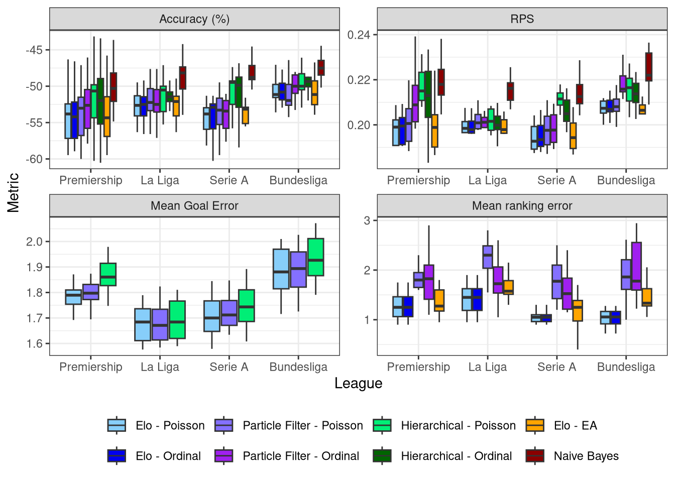
It highlights some interesting patterns that were hidden in the overall table:
- RPS shows more variability than accuracy and is therefore more useful as evaluator of models. Not least because predicting sports matches is often used to aid in betting, which necessitates probabilities
- In the RPS plot we can see that the hierarchical models generally are the least accurate, except in La Liga where they perform very similarly to the time-based systems. This suggests that teams skill levels aren’t changing as much as they are in other leagues. It’s no shock that the top 2 in Spain don’t change, but it’s a surprise to see evidence for it happening across the entire league
- The particle filters do proportionally worse in their team ratings than their match predictions. I think this is the cause of their surprisingly low match predictive accuracy - their rating updates are hampered by the state updating issues which weakens the downstream match predidctions. If the particle filters can be optimized to smooth the state estimation then I think their match prediction accuracy will bounce back
- We can more clearly see that the Poisson particle filter outperforms the ordinal varient across the board
- The mean goal error is relatively consistent between models at 1.6 - 2.0. This seems slightly higher than I’d anticipate - I feel on average a human would be within 2 goals of the correct scoreline - would it be enough to use as a basis for score betting?
Conclusion
In conclusion then, well done to the standard Elo rating system with the Poisson classifier! If I ever decide to pick this up again I have two further avenues for exploration which are quite different in their approach:
- Statistical: Optimizing the particle filters
- Data driven: Using a neural network
The particle filters have been hindered by my naive application, and have performed quite well in spite of some model mispecifcations. If I can get the states updating smoothly without updating teams who aren’t playing (probably by implementing a guided filter), and PMMH working well, then I think these models could be quite accurate. I value having a formal probabilistic specification which provides uncertainty estimates and I appreciate the conciseness of the models - they are completely defined by 2 priors and a likelihood function - and the fact that the rating update is abstracted away entirely. However, the simple Elo rating system performs so well that it begs for additional attention. The EA model should have been tested with a Poisson outcome for a start, and a neural network replacing the hardcoded rating and prediction functions will be far more flexible and scale far better to new leagues and sports.
Watch this space…