Predictaball retrospective part 4 - Particle Filters

Jan 22, 2026 36 min read

Introduction

This is the fourth in a series of posts looking back at the various statistical and machine learning models that have been used to predict football match outcomes as part of Predictaball. Here’s a quick summary of the first 3 parts:

Part 1 used a Bayesian hierarchical regression to model a team’s latent skill, where skill was constant over time
Part 2 used an Elo rating system to handle time, but the functions and parameters were hardcoded and a match prediction model was bolted on top to replace Elo’s basic prediction
Part 3 used Evolutionary Algorithms (EA) to simultaneously optimize the rating system and match prediction model without requiring any hardcoding parameters

The EA model has working reliably for the last 5 and a half seasons and hasn’t been tweaked since. However, I still prefer a fully probabilistic model when possible so I wanted to revisit the Bayesian model and extend it to the time domain.

Particle Filters

State-space models are one of the most well known techniques for modelling time-series data within a probabilistic framework. They are parameterised by observed data $y$ and latent states $x$ and their behaviour is governed by two equations:

One that links the observed data to the latent states: $y_t = f(x_t)$
Another that defines how the states evolve over time: $x_{t+1} = g(x_t)$

Where $f(.)$ and $g(.)$ generally incorporate stochastic elements. I.e. in the most general linear Gaussian case, where $A$ and $C$ are matrices:

$$y_t = Ax_t + \epsilon_t$$ $$x_{t+1} = Cx_t + \eta_t$$

And

$$\epsilon_t \sim \text{Normal}(0, \sigma_\epsilon)$$ $$\eta_t \sim \text{Normal}(0, \sigma_\eta)$$

I’ve used linear Gaussian state-space filters a fair bit in my work on analysing air quality trends as they are incredibly flexible and very fast to implement with the Kalman filter. However, the Kalman filter only handles Gaussian likelihoods and priors. My previous regression modelling used Poisson and Ordinal Logistic likelihoods and I’d like to use these again instead of hacking a Gaussian distribution for football modelling.

There is a more flexible variety of state-space models, called Particle Filters, which do not make any such requirements. Particles filters are also known as ‘Sequential Monte Carlo’, which gives a clue as to their functionality. They sequentially make Monte Carlo draws to estimate the posterior parameters given some priors and a likelihood function using a pool of random chains (‘particles’). My reference for particle filters (IMO a far better name than SMC from a PR perspective) is the excellent book by Chopin & Papaspiliopoulous, who also published a Python package that accompanies the book.

I’ve been investigating using these for my day job and realised their flexibility makes them very applicable for football prediction too. The downside of this flexibility as always is in computational cost: without an analytical solution like the Kalman filter they have to use a Monte Carlo search which is far more expensive.

In this post I’ll demonstrate how I’ve applied them for this purpose - the first new model development on Predictaball in 6 years, so I’m very excited!

Setup

As might be obvious, I very much prefer R to Python for routine data analysis: I like the tidyverse’s more friendly SQL-like syntax, its integration with many data sources via dbplyr saves learning different APIs, and I much prefer RStudio and Quarto notebooks to Jupyter. That’s not even going into how ggplot2 blows matplotlib out of the water for both usability and attractiveness. However, I am pragmatic and will use Python when it’s the best choice, which is the case here as the authors of the Particle Filters book that I mentioned that I’m using have written an excellent Python package particles to accompany the book.

However, I will still be a bit awkward and refuse to dip my toes entirely into Python land and instead will work in Quarto. This allows me to use the same IDE I use for my R analysis with all of my keybinds setup (hooray for Vim mode) as well as allowing data to be shared between the 2 environments (i.e. I can do all my data munging with glorious tidyverse/SQL syntax and plot with ggplot2, while using Python libraries for the actual computation). The introduction of uv in particular has massively helped this by allowing you to just state your Python requirements for reticulate (the R -> Python wrapper) to create an ephemeral environment for you behind the scenes. Magic.

Show the code


Sys.setenv("RETICULATE_USE_MANAGED_VENV"="yes")
library(reticulate)
py_require(
    c(
        "particles==0.4",
        "pandas==2.3.3",
        "numpy",
        "scipy",
        "matplotlib",
        "seaborn"
    ),
    python_version = ">=3.13"
)
library(tidyverse)
library(knitr)
library(kableExtra)
library(ggrepel)
library(latex2exp)
options(knitr.table.html.attr = "quarto-disable-processing=true")

The Python packages that will be needed are straightforward, outside of all the particles imports (another thing R does better than Python IMO is loading libraries, submodules are a great idea in theory for namespacing but can quickly pollute user code).

Show the code


import particles
from particles import mcmc
from particles import smc_samplers as ssp
import particles.state_space_models as ssm
import particles.distributions as dists
from particles.collectors import Moments
import pandas as pd
from scipy.stats import norm, poisson

import matplotlib.pyplot as plt
from time import time
import seaborn as sb
import pickle
import numpy as np

Show the code


def inv_logit(x):
    return 1 / (1 + np.exp(-x))

And now to just setup the dataset, pulling the dataframe across from R (again, reticulate is magic). Although hang on, is that the dreaded global keyword rearing its head against all best practices? Er yes, it will make sense soon, I swear.

Show the code


global home_ids
global away_ids
global N_teams
df = r.df.loc[
    (r.df['league'] == 'premiership') & (r.df['dset'] == 'training'), 
    ['matchid', 'home', 'away', 'home_score', 'away_score', 'result', 'date']
]
df['home_id'] = df['home'].astype('category').cat.codes
df['away_id'] = df['away'].astype('category').cat.codes
home_ids = df['home_id'].values
away_ids = df['away_id'].values
N_teams = np.unique(home_ids).size

Poisson model of goals scored

Back to the whiteboard of maths a second to describe the models we’ll be using. The likelihood is the exact same as in the hierarchical model, with a Poisson distribution whose rate is composed of an intercept (average number of goals scored) and the difference between the 2 teams’ skill levels: $\psi_\text{team}$. The only difference with the hierarchical regression is that there is now an additional subscript $t$ indicating that a team’s skill varies over time.

$$\text{goals}_\text{home} \sim \text{Poisson}(\lambda_{\text{home},i,t})$$ $$\text{goals}_\text{away} \sim \text{Poisson}(\lambda_{\text{away},i,t})$$

$$\log(\lambda_{\text{home},i,t}) = \alpha_{\text{home},\text{leagues[i]}} + \psi_\text{home[i],t} - \psi_\text{away[i],t}$$ $$\log(\lambda_{\text{away},i,t}) = \alpha_{\text{away},\text{leagues[i]}} + \psi_\text{away[i],t} - \psi_\text{home[i],t}$$

This is because $\psi_t$ is going to be the unobserved latent state in our state-space model and we assume it evolves over time. Our prior on it will be a random walk with a given variance $\sigma_\psi$, which will determine how much each teams’ ratings are updated post-match.

$$\psi_\text{home[i],t} \sim \text{Normal}(\psi_\text{home[i],t-1}, \sigma_\psi)$$

The final prior needed to complete the state-space model definition is the prior $\psi_0$ - how the initial values are distributed. This took some work to get right, as initially I used a generic uninformative prior $\text{Normal}(0, 2.5)$, but it wasn’t producing sensible results. Instead, I had to start all teams at the same place i.e. with 0 (mean) skill as otherwise the model wasn’t able to get into a sensible starting position as it assumed the randomly drawn skills were meaningful.

$$\psi_\text{home[i],0} \sim \text{Dirac}(0)$$

How this looks in code is shown below. I think this class definition nicely illustrates how straight forward and user friendly particles is. You only have to define 3 functions with straight forward parameterisations and can do whatever you want within those functions (you could even have the states be weights in a multi-layer perceptron (MLP) but it will struggle to filter) using standard Python data types. I contrast this with my Stan experiences where every time I come to write a new model I am constantly consulting the docs to remind myself the syntax for declaring constraints or when to use array vs vector vs matrix etc…

However that said, there was still a fair bit of trial and error to get to this point and I’d be remiss if I pretended otherwise. In particular, things that tripped me up:

Because of the multivariate output, all parameters had to be 2D
The intercept needed to be hardcoded as a parameter rather than used as a state
Initially for PX I didn’t have the conditional Dirac prior, which meant that all teams’ skill got updated after every match, not just those that played
As mentioned, I initially was setting $\psi_0 \sim \text{Normal}(0, 2.5)$ in the classic state-space manner. But this was too strong a prior as it affected the football prediction results and the system couldn’t settle. This was fixed by forcing every team’s skill to start at 0 using a Dirac distribution
The methods are parameterised only in terms of time and the states, so if you want to bring outside information in (such as which team is playing the current match), this needs to be brought in via global variables, hence defining them above

Show the code


class PoissonModel(ssm.StateSpaceModel):
    def PX0(self):  # Distribution of X_0 
        return dists.IndepProd(
            *[dists.Dirac(loc=0) for _ in range(N_teams)]
        )
    def PX(self, t, xp):  # Distribution of X_t given X_{t-1}
        # update X either as random walk if was playing else don't change
        distributions = [
            dists.Normal(
                loc=xp[:, i],
                scale=self.skill_walk_variance
            ) 
            if i == home_ids[t] or i == away_ids[t] 
            else dists.Dirac(loc=xp[:, i]) 
            for i in range(N_teams)
            ]
        return dists.IndepProd(*distributions)
    
    def PY(self, t, xp, x):  # Distribution of Y_t given X_t (and X_{t-1}) 
        lp_home = np.exp(
            self.home_intercept + x[:, (home_ids[t])] - x[:, (away_ids[t])]
        )
        lp_away = np.exp(
            self.away_intercept + x[:, (away_ids[t])] - x[:, (home_ids[t])]
        )
        return dists.IndepProd(
            dists.Poisson(rate=lp_home),
            dists.Poisson(rate=lp_away)
        )

Now we can instantiate a model by providing those 3 parameters: $\alpha_\text{home}, \alpha_\text{away}, \sigma_\psi$. We know from previous analysis that roughly the home team scores 1.5 goals on average and the away 1.2. For $\sigma_\psi$ let’s just use a low value (0.01) and see how this impacts the ratings. The filter itself ran quickly, which is always a bonus when dealing with anything Monte Carlo.

Show the code


mod1 = PoissonModel(
    home_intercept=np.log(1.5),
    away_intercept=np.log(1.2),
    skill_walk_variance=0.01
)
filt1 = particles.SMC(
    fk=ssm.Bootstrap(ssm=mod1, data=df[['home_score', 'away_score']].values),
    N=1000,
    collect=[Moments()]
)
a = time()
filt1.run()
b = time()

# Save final rating skills
scores = df[['home', 'home_id']].drop_duplicates().sort_values('home_id')
scores['score'] =  filt1.summaries.moments[df.shape[0]-1]['mean']

print(f"Time taken: {b-a}s")

Time taken: 3.953542709350586s

The final ratings at the end of the training period (2005-2006 season up to 2014-2015) are shown below. Interestingly the ratings have both Man City and Man Utd above Chelsea: the league winners. However, it must be remembered that in this Poisson model $\psi$ doesn’t correspond directly to a team’s strength at winning a match but rather scoring a goal. And if we look at the goal difference for this season we can see that actually Man City topped the group with +45, whereas Chelsea were in second with +41, so maybe this isn’t isn’t as odd as it first seems. Otherwise it seems generally accurate, although Everton are ranked quite a bit higher than their final league position, and it’s not like they had a particularly strong goal scoring record (they were 9th on Goal Difference).

Show the code


league_positions_training <- tribble(
    ~position, ~team,
    1, "Chelsea",
    2, "Man City",
    3, "Arsenal",
    4, "Man Utd",
    5, "Tottenham",
    6, "Liverpool",
    7, "Southampton",
    8, "Swansea",
    9, "Stoke",
    10, "Crystal Palace",
    11, "Everton",
    12, "West Ham",
    13, "West Brom",
    14, "Leicester",
    15, "Newcastle",
    16, "Sunderland",
    17, "Aston Villa",
    18, "Hull",
    19, "Burnley",
    20, "QPR"
)
tab_df <- py$scores |>
    as_tibble() |>
    rename(team=home) |>
    inner_join(
        league_positions_training, by="team"
    ) |>
    arrange(desc(score)) |>
    mutate(rank_skill = row_number()) |>
    select(team, score, rank_skill, position) |>
    mutate(difference = abs(position - rank_skill)) 

tab_df |>
    kable("html", align=c("l", "c", "c", "c", "c"), digits=3, col.names = c("Team", "Skill", "Rank", "Final league position", "Difference"), row.names = FALSE) |>
    kable_styling(c("striped", "hover"), full_width=F) |>
    column_spec(
        5, color = ifelse(tab_df$difference == 0, 'green', 'red')
    )

Team	Skill	Rank	Final league position	Difference
Man City	0.424	1	2	1
Man Utd	0.381	2	4	2
Chelsea	0.381	3	1	2
Arsenal	0.370	4	3	1
Liverpool	0.243	5	6	1
Everton	0.208	6	11	5
Tottenham	0.175	7	5	2
Southampton	0.132	8	7	1
Crystal Palace	0.063	9	10	1
Leicester	0.023	10	14	4
Swansea	0.021	11	8	3
West Ham	0.011	12	12	0
Stoke	-0.050	13	9	4
Burnley	-0.051	14	19	5
West Brom	-0.053	15	13	2
Hull	-0.074	16	18	2
Sunderland	-0.149	17	16	1
QPR	-0.151	18	20	2
Newcastle	-0.174	19	15	4
Aston Villa	-0.176	20	17	3

The ratings over the full training data period from 2005 to 2014 are shown in Figure 1. They generally look quite reasonable, e.g. we can see the “big 6” (and Everton!) separated from the rest of the pack. Interestingly there seems to be a big change between the 2009-2010 and 2010-2011 seasons - possible shock to teams’ finances following the crash?

Show the code


scores1 <- map_dfr(py$filt1$summaries$moments, function(x) {
    x |> 
        as_tibble() |>
        mutate(teamid = row_number()-1)
}) |>
    mutate(
        date = rep(
            df |> 
                filter(league == 'premiership', dset == 'training') |> 
                pull(date), 
            each=py$N_teams
            )
    ) |>
    inner_join(
        py$df |>
            distinct(home, home_id),
        by=c("teamid"="home_id")
    )

Show the code


teams_all_seasons <- df |> 
    filter(league == 'premiership', dset == 'training') |> 
    distinct(season, home) |> 
    count(home) |>
    filter(n >= 7)

plt_df <- scores1 |>
    filter(date >= as_date('2005-09-01')) |>
    inner_join(teams_all_seasons)

lab_df <- plt_df |>
    group_by(home) |>
    filter(date == max(date)) |>
    summarise(
        date = mean(date),
        mean = mean(mean)
    ) |>
    ungroup()

seasons <- df |>
    filter(league == 'premiership', dset == 'training') |> 
    group_by(season) |>
    summarise(start = min(date), end=max(date)) |>
    ungroup()

plt_df |>
    ggplot() +
        geom_rect(aes(xmin=start, xmax=end), ymin=-Inf, ymax=Inf,
                  data=seasons, fill='lightblue', alpha=0.3) +
        geom_line(aes(x=date, y=mean, colour=home)) +
        theme_minimal() +
        geom_label_repel(aes(x=date, y=mean, label=home, colour=home), hjust=0, data=lab_df,
                         max.overlaps = 20) +
        scale_x_datetime(
            expand=expansion(mult=c(0, 0.3)),
            breaks=seq.POSIXt(
                from=as_datetime("2006-01-01"),
                to=as_datetime("2015-01-01"),
                by="1 year"
            ),
            labels=c(
                "2005-2006",
                "2006-2007",
                "2007-2008",
                "2008-2009",
                "2009-2010",
                "2010-2011",
                "2011-2012",
                "2012-2013",
                "2013-2014",
                "2014-2015"
            )
        ) +
        guides(colour="none") +
        theme(
            legend.position = "bottom",
            axis.text.x = element_text(angle=45, hjust=1) 
        ) +
        labs(x="", y=TeX("Modelled skill $\\psi$$"))

$Estimated $\psi$ over the course of the training set$

Figure 1: Estimated $\psi$ over the course of the training set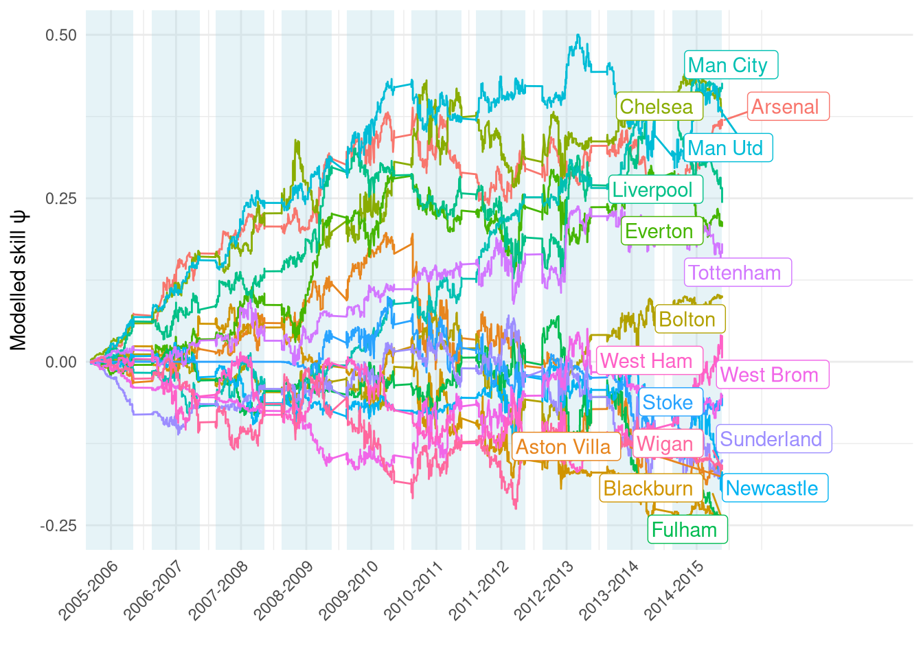

Figure 2 zooms in to the 2014-2015 season for 3 select teams (Burnley, Man City, Chelsea) to have a closer look. While we can see the step changes after each match, the overall changes look quite small which is good - we wouldn’t want to see a team having large updates after each match as that would add noise masking the longer-term trend. We can also see that Chelsea’s rating decreasing in the second half of the season which makes sense as they won the league quite comfortably with 3 games to spare, meanwhile we can see City finishing strong.

Show the code


scores1 |>
    filter(
        date >= as_date('2014-09-01'),
        home %in% c('Man City', 'Chelsea', 'Burnley')
    ) |>
    mutate(
        lower = mean - 2 * sqrt(var),
        upper = mean + 2 * sqrt(var)
    ) |>
    ggplot(aes(x=date, y=mean)) +
        geom_ribbon(aes(ymin=lower, ymax=upper), alpha=0.5, fill='steelblue') +
        geom_line() +
        facet_wrap(~home) +
        theme_minimal() +
        theme(
            legend.position = "bottom"
        ) +
        labs(x="", y=TeX("Modelled skill $\\psi$"))

Figure 2: Modelled rating for 3 teams in the 2014-2015 season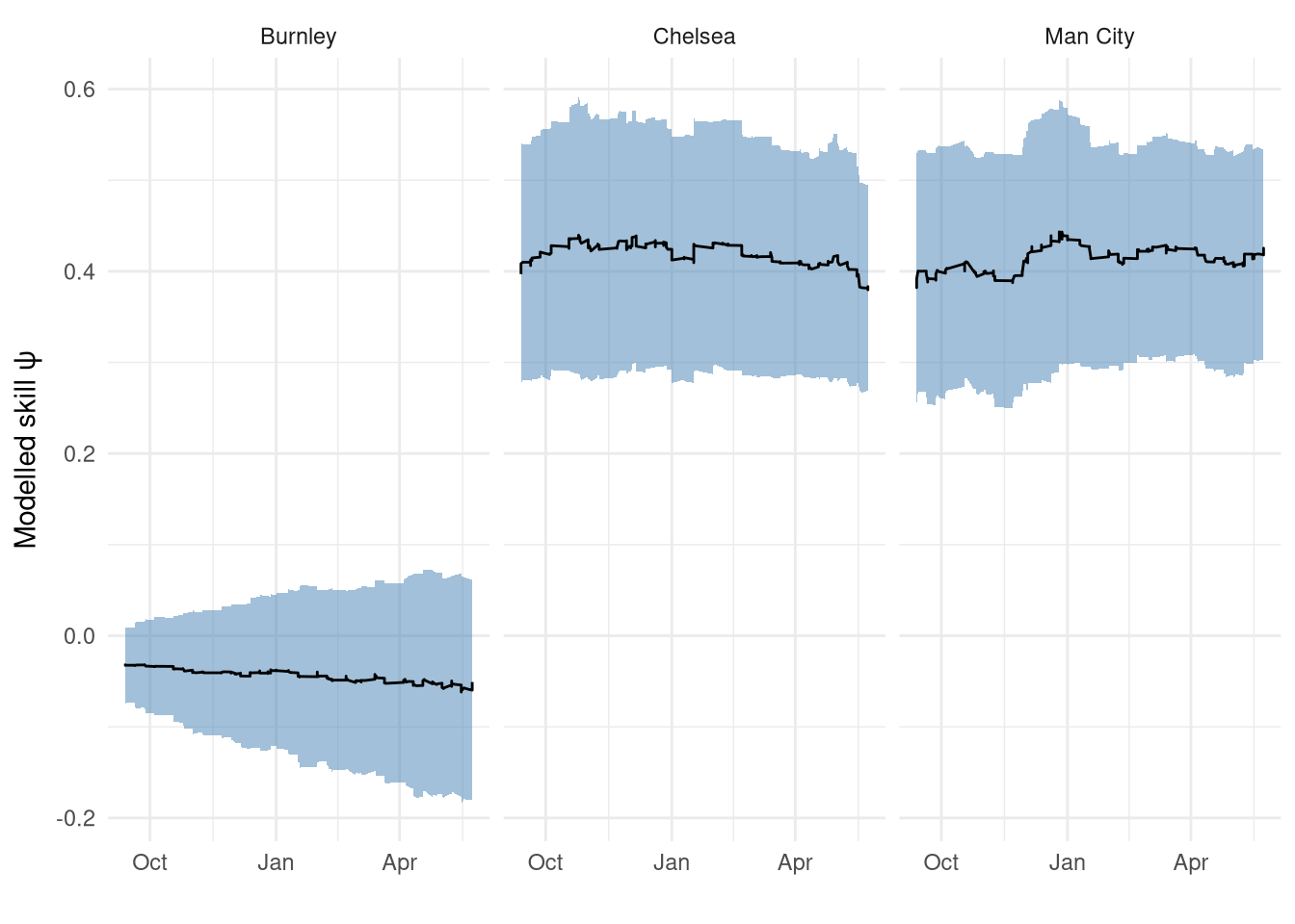

The only problem with this model that isn’t obvious from these time-series is that team’s ratings are still being updated even when they aren’t playing matches. Generally these are little updates that suggest it’s just variance between the particles, but in some more egregious cases it’s more substantial. For example, in this training period, Reading had 2 spells in the Premiership between 2006-2008 and then during the 2012-2013 campaign. However, Figure 3 shows that Reading’s skill level is being updated when they aren’t even in the Premiership. I suspect this isn’t an issue with Particle Filters themselves, but how I’m using this particular software implementation. I’ll likely need to use a more manual approach, either using a custom model (not the SSM convenience class that particles provides around the underlying Feynman-Koch model), exploring the array of different Particle Filter configurations available (I’m just using the basic Bootstrap Filter), or my own implementation bespoke for this applicatoin.

Show the code


scores1 |>
    filter(home == 'Reading') |>
    mutate(
        lower = mean - 2 * sqrt(var),
        upper = mean + 2 * sqrt(var)
    ) |>
    ggplot(aes(x=date, y=mean)) +
        annotate("rect", ymin=-Inf, ymax=Inf, xmin=as_date("2006-08-01"), xmax = as_date("2008-08-01"), alpha=0.4, fill='forestgreen') +
        annotate("label", x=as_date("2006-08-01"), y=0.2, label="In Premiership", hjust=0, fill="forestgreen", colour="white") +
        annotate("rect", ymin=-Inf, ymax=Inf, xmin=as_date("2012-08-01"), xmax = as_date("2013-08-01"), alpha=0.4, fill='forestgreen') +
        annotate("label", x=as_date("2012-08-01"), y=0.2, label="In Premiership", hjust=0, fill="forestgreen", colour="white") +
        geom_ribbon(aes(ymin=lower, ymax=upper), alpha=0.5, fill='steelblue') +
        geom_line() +
        theme_minimal() +
        theme(
            legend.position = "bottom"
        ) +
        labs(x="", y=TeX("Modelled skill $\\psi$"))

Figure 3: Reading’s skill change between 2005-2015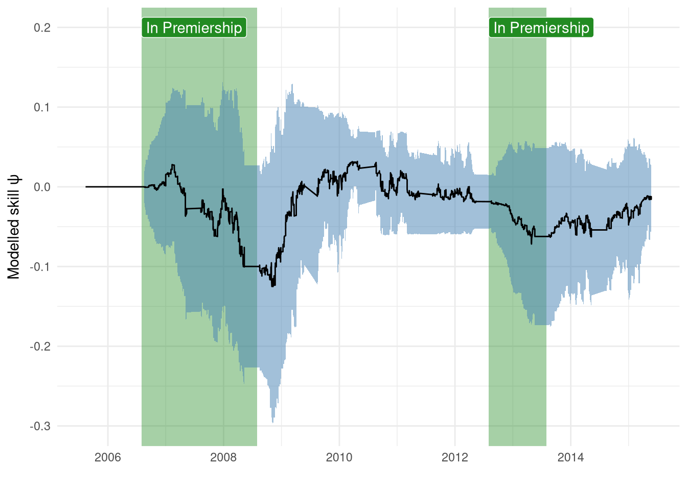

Bayesian parameter inference - PMMH

In the first model the three parameters ($\alpha_\text{home}, \alpha_\text{away}, \sigma_\psi$) were hardcoded to somewhat sensible values. Particle marginal Metropolis-Hastings is a way of estimating these parameters for a state-space model that uses particle filters to sample the posterior. This is relatively slow, taking around 25 minutes to run with the parameters below. I used an uninformative prior on $\sigma_\psi$ as I have little intuition what that value should be, but for the $\alpha$ we would expect them to be very similar to the values we’ve used in the past: the raw goal scoring rate for each side from the data. I’ve kept a relatively wide variance for these just to not limit the search too much, particularly since there is a decent amount of data (14k matches) that the posterior shouldn’t be swayed too much by the prior.

Show the code


prior_dict = {
    'skill_walk_variance': dists.LogNormal(mu=0, sigma=1),
    'home_intercept': dists.Normal(loc=np.log(1.5), scale=2),
    'away_intercept': dists.Normal(loc=np.log(1.2), scale=2),
}
prior_1 = dists.StructDist(prior_dict)

Show the code


pmmh_1 = mcmc.PMMH(
    ssm_cls=PoissonModel,
    prior=prior_1,
    data=df[['home_score', 'away_score']].values,
    Nx=200,     # N particles
    niter=1000  # MCMC iterations
)
a = time()
pmmh_1.run(); 
b = time()
pmmh_1_df = pd.DataFrame(pmmh_1.chain.theta)

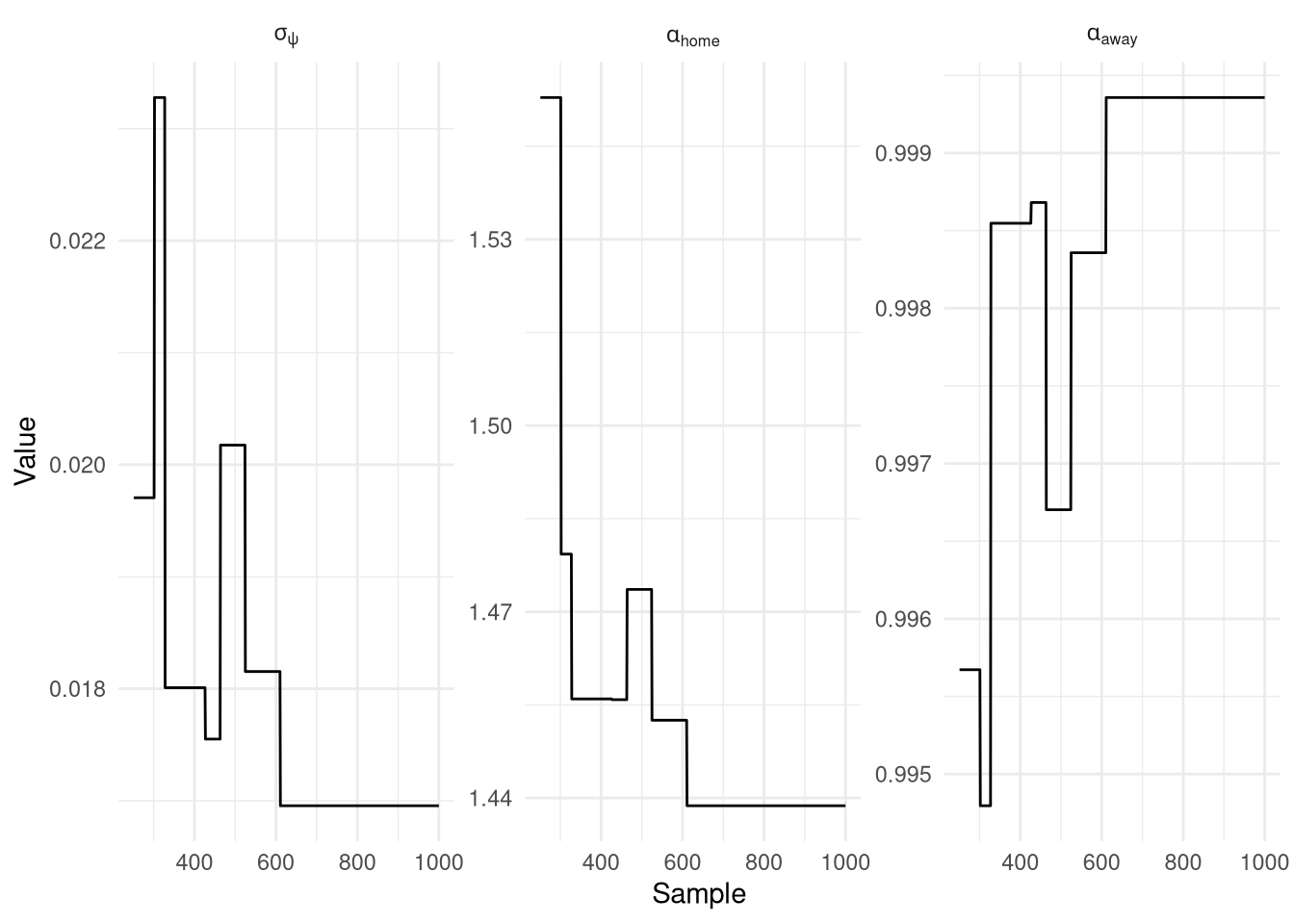
The results of the 1,000 iterations (minus the first 250 for burn-in) are plotted below in Figure 4, and confusingly unlike any MCMC trace I’ve seen before, these are completely flat! The values themselves look sensible ($\alpha_\text{home}=1.44, \alpha_\text{away}=1$), but there is no variance at all. I suspect this might be due to the awkward Dirac priors I’ve used to try and only update the skill of the teams playing the match, rather than all teams. $\sigma_\psi = 0.017$, which actually isn’t that far off the naive guess of 0.01 that I used previously.

Show the code


py$pmmh_1_df |>
    mutate(
        sample = row_number(),
        home_intercept = exp(home_intercept),
        away_intercept = exp(away_intercept),
    ) |>
    filter(sample > 250) |>  # Remove burn-in
    pivot_longer(-sample) |>
    mutate(
        name = factor(
            name,
            levels=c("skill_walk_variance", "home_intercept", "away_intercept"),
            labels=c(TeX("$\\sigma_\\psi$"), TeX("$\\alpha_{home}$"), TeX("$\\alpha_{away}$"))
        )
    ) |>
    ggplot(aes(x=sample, y=value)) +
        geom_line() +
        facet_wrap(~name, scales="free", labeller=label_parsed) +
        theme_minimal() +
        labs(x="Sample", y="Value")

Figure 4: PMMH traces

So let’s see how these values (well really $\sigma_\psi$ since $\alpha$ has barely changed) impacts on the ratings. A new model is fitted using the parameters estimated by PMMH, and as usual the filtering itself is fast.

Show the code


# These are the parameter values identified by PMMH
mod2 = PoissonModel(
    home_intercept=np.log(1.44),
    away_intercept=np.log(1),
    skill_walk_variance=0.017
)
filt2 = particles.SMC(
    fk=ssm.Bootstrap(
        ssm=mod2,
        data=df[['home_score', 'away_score']].values
    ),
    N=1000,
    collect=[Moments()]
)
a = time()
filt2.run()
b = time()
print(f"Time taken: {b-a}s")

Time taken: 3.304931163787842s

Figure 5 compares the ratings time-series for both models. The higher $\sigma_\psi$ from the PMMH model allows the ratings to fluctuate far more, making the ratings more influenced by the latest match than the long-term trend. It also means that those longer-term trends are even stronger, i.e. the gap between the top and bottom teams is even more pronounced now.

Show the code


scores2 <- map_dfr(py$filt2$summaries$moments, function(x) {
    x |> 
        as_tibble() |>
        mutate(teamid = row_number()-1)
}) |>
    mutate(
        date = rep(
            df |> 
               filter(league == 'premiership', dset == 'training') |>
               pull(date), 
            each=py$N_teams
        )
    ) |>
    inner_join(
        py$df |>
            distinct(home, home_id),
        by=c("teamid"="home_id")
    )

plt_df <- scores1 |>
    mutate(method="Hardcoded") |>
    rbind(scores2 |> mutate(method = "PMMH")) |>
    filter(date >= as_date('2005-09-01')) |>
    inner_join(teams_all_seasons)


lab_df <- plt_df |>
    group_by(home, method) |>
    filter(date == max(date)) |>
    summarise(
        date = mean(date),
        mean = mean(mean)
    ) |>
    ungroup()

plt_df |>
    ggplot() +
        geom_rect(aes(xmin=start, xmax=end), ymin=-Inf, ymax=Inf,
                  data=seasons, fill='lightblue', alpha=0.3) +
        geom_line(aes(x=date, y=mean, colour=home)) +
        theme_minimal() +
        facet_wrap(~method) +
        geom_label_repel(aes(x=date, y=mean, colour=home, label=home), hjust=0, data=lab_df,
                         max.overlaps = 20) +
        scale_x_datetime(
            expand=expansion(mult=c(0, 0.3)),
            breaks=seq.POSIXt(
                from=as_datetime("2006-01-01"),
                to=as_datetime("2015-01-01"),
                by="1 year"
            ),
            labels=c(
                "2005-2006",
                "2006-2007",
                "2007-2008",
                "2008-2009",
                "2009-2010",
                "2010-2011",
                "2011-2012",
                "2012-2013",
                "2013-2014",
                "2014-2015"
            )
        ) +
        guides(colour="none") +
        theme(
            legend.position = "bottom",
            axis.text.x = element_text(angle=45, hjust=1)
        ) +
        labs(x="", y=TeX("Modelled skill $\\psi$"))

$Comparison of $\psi$ between filter parameters manually selected or estimated via PMMH$

Figure 5: Comparison of $\psi$ between filter parameters manually selected or estimated via PMMH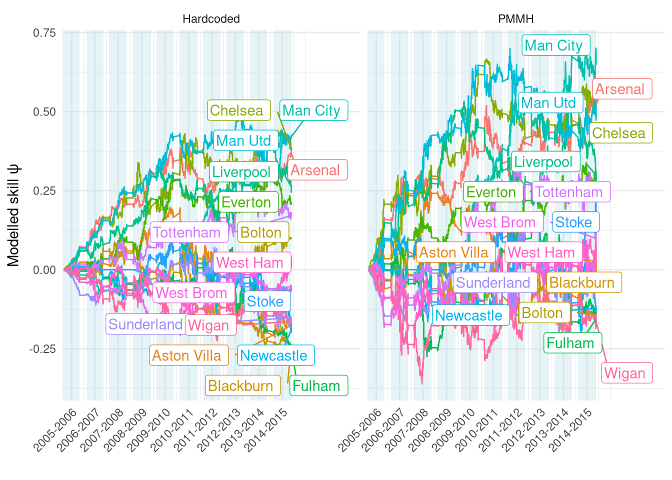

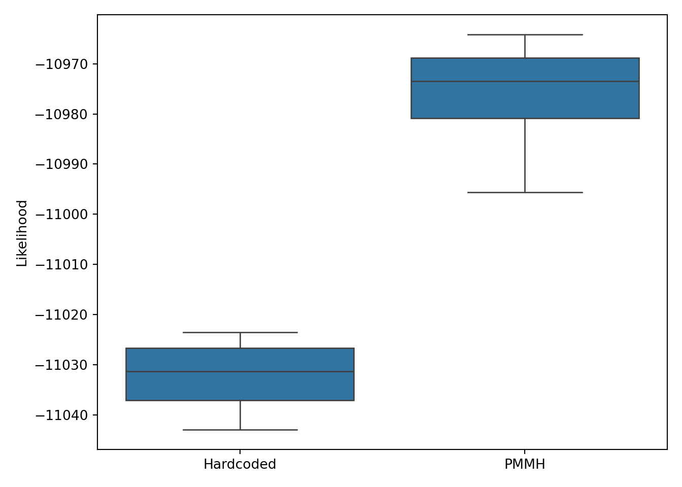
By eye I prefer the PMMH ratings as it allows for a quicker response to a change in a team’s performance (which often can hinge on one injury or manager change) without looking too filled with short-term noise. But can we quantifiably compare models to see which fits best? Yes, we can do so easily using a likelihood comparison as both models are fully probabilistic with the same likelihood formulation. The log-likelihoods from 10 runs are shown in Figure 6, demonstrating a clear preference for the parameters estimated using PMMH.

Show the code


res_hardcoded = particles.multiSMC(
    fk=ssm.Bootstrap(
        ssm=mod1,
        data=df[['home_score', 'away_score']].values
    ),
    N=1000,
    nruns=10
)

res_auto = particles.multiSMC(
    fk=ssm.Bootstrap(
        ssm=mod2,
        data=df[['home_score', 'away_score']].values
    ),
    N=1000,
    nruns=10
)
res_df = pd.DataFrame({
    'res': [r['output'].logLt for r in res_hardcoded] + [r['output'].logLt for r in res_auto],
    'group': ['Hardcoded']*10 + ['PMMH']*10
})
plt.clf()
ax = sb.boxplot(res_df, x='group', y='res')
ax.set(xlabel='', ylabel='Likelihood')
plt.tight_layout()
plt.show()

Figure 6: Comparison of the two filters using hardcoded parameters vs values estimated via PMMH on their likelihood

Increasing skill variance at the start of the season

A lot can change in the summer off-season, as highlighted in Figure 1 where it seemed some teams had a large rating change between the end of the 2009-2010 and the start of the 2010-2011 season. This was handled in the Elo model by lowering everyone’s skill by 20% at the start of the season, and ideally a similar correction would be incorported into this particle filter model. One idea I had was to temporarily increase $\sigma_\psi$ at the start of the season to allow ratings to adjust more quickly. In particular, I wanted to double $\sigma_\psi$ in the first 5 matches of the season.

I first need to generate fields that track how many teams either side has played (again this is a pure data munging task that is far easier in R/tidyverse than Pandas).

Show the code


home_games <- df |> 
    distinct(matchid, season, date, team=home, league)
away_games <- df |> 
    distinct(matchid, season, date, team=away, league)
matches_in_season <- home_games |>
    rbind(away_games) |>
    arrange(league, season, team, date) |>
    group_by(league, season, team) |>
    mutate(match_of_season = row_number()) |>
    ungroup() |>
    select(matchid, team, match_of_season)

df2 <- py$df |>
    inner_join(
        matches_in_season |> 
            rename(home=team, home_match_of_season=match_of_season),
       by=c("matchid", "home")
    ) |>
    inner_join(
        matches_in_season |>
            rename(away=team, away_match_of_season=match_of_season),
        by=c("matchid", "away")
    ) |>
    mutate(
        result_int = as.integer(
            factor(
                result, 
                levels=c("away", "draw", "home")
            )
        )
    )

This change will be reflected in the PX method, which is the one that governs how the states are updated from the previous timepoint. The logic was already getting a bit long for 1 method owing to the conditional logic to use a Dirac distribution to keep rating constant for teams that hadn’t played, so I’ll refactor it out into its own function. Again we’ll need to expose the number of matches each team has played via a global variable as there’s no other way of passing this information into the filter.

Show the code


global home_season_matches
global away_season_matches
global home_ids
global away_ids
home_ids = r.df2['home_id'].values
away_ids = r.df2['away_id'].values
home_season_matches = r.df2['home_match_of_season'].values
away_season_matches = r.df2['away_match_of_season'].values

def get_team_PX(xp, t, team_id, var):
    if home_ids[t] == team_id:
        mult = 2 if home_season_matches[t] < 5 else 1
        return dists.Normal(loc=xp, scale=mult * var)
    elif away_ids[t] == team_id:
        mult = 2 if away_season_matches[t] < 5 else 1
        return dists.Normal(loc=xp, scale=mult * var)
    else:
        return dists.Dirac(loc=xp)

Then the new StateSpaceModel refers to this function in its PX method - it is otherwise identical to PoissonModel.

Show the code


class PoissonModelDoubleVariance(ssm.StateSpaceModel):
    def PX0(self):  # Distribution of X_0 
        return dists.IndepProd(
            *[dists.Dirac(loc=0) for _ in range(N_teams)]
        )
    def PX(self, t, xp):  # Distribution of X_t given X_{t-1}
        distributions = [
            get_team_PX(
                xp[:, i],
                t,
                i,
                self.skill_walk_variance
            ) 
            for i in range(N_teams)
        ]
        return dists.IndepProd(*distributions)
    
    def PY(self, t, xp, x):  # Distribution of Y_t given X_t (and X_{t-1}) 
        lp_home = np.exp(
            self.home_intercept + x[:, (home_ids[t])] - x[:, (away_ids[t])]
        )
        lp_away = np.exp(
            self.away_intercept + x[:, (away_ids[t])] - x[:, (home_ids[t])]
        )
        return dists.IndepProd(
            dists.Poisson(rate=lp_home),
            dists.Poisson(rate=lp_away)
        )

I’ll make 2 filters here, one with the initial hardcoded parameter values and the other using those identified using PMMH (albeit on the model with constant $\sigma_\psi$).

Show the code


# These are the manually chosen parameter values
mod3 = PoissonModelDoubleVariance(
    home_intercept=np.log(1.5),
    away_intercept=np.log(1.2),
    skill_walk_variance=0.01
)
filt3 = particles.SMC(
    fk=ssm.Bootstrap(
        ssm=mod3,
        data=r.df2[['home_score', 'away_score']].values
    ),
    N=1000,
    collect=[Moments()]
)

# These are the parameter values identified by PMMH on the model that didn't
# use a multiplier at the start of the season
mod4 = PoissonModelDoubleVariance(
    home_intercept=np.log(1.44),
    away_intercept=np.log(1),
    skill_walk_variance=0.017
)
filt4 = particles.SMC(
    fk=ssm.Bootstrap(
        ssm=mod4,
        data=r.df2[['home_score', 'away_score']].values
    ),
    N=1000,
    collect=[Moments()]
)
a = time()
filt3.run()
filt4.run()
b = time()
print(f"Time taken: {b-a}s")

Time taken: 7.586232900619507s

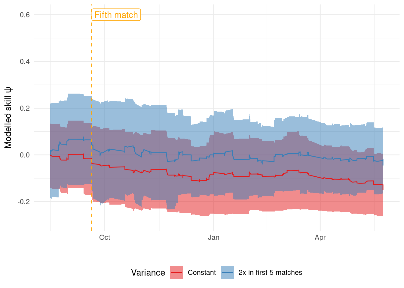
The rating changes from both filters for a single team (Liverpool) over a single season are shown in Figure 7. I was hoping to see a far jumpier signal in the first 5 games for the double variance model but it only seems to be a little different at best. The main difference is the rating value they settle on, whereas I was expecting them to get to the same level at different rates. This highlights nicely that there is considerable variance between particle filter runs, which is why it’s important to take this into account.

Show the code


five_match_date <- df2 |>
    mutate( date = as_date(unlist(date))) |>
    filter(
        date >= '2014-08-01', date < '2015-08-01',
        (home == 'Liverpool' & home_match_of_season == 5) | (away == 'Liverpool' & away_match_of_season == 5)
    ) |>
    pull(date)

scores3 <- map_dfr(py$filt3$summaries$moments, function(x) {
    x |> 
        as_tibble() |>
        mutate(teamid = row_number()-1)
}) |>
    mutate(date = rep(df2 |> pull(date), each=py$N_teams)) |>
    inner_join(
        df2 |>
            distinct(home, home_id),
        by=c("teamid"="home_id")
    ) |>
    mutate(date = as_date(unlist(date)))

scores1 |>
    filter(home == 'Liverpool') |>
    mutate(
        model = 'static'
    ) |>
    rbind(
        scores3 |>
            mutate(model = 'double')
    ) |>
    filter(home == 'Liverpool', date >= '2014-08-01', date < '2015-08-01') |>
    arrange(date) |>
    group_by(model) |>
    mutate(
        start_mean = mean[1]  
    ) |>
    ungroup() |>
    mutate(
        mean = mean - start_mean,
        lower = mean - 2 * sqrt(var),
        upper = mean + 2 * sqrt(var),
        model = factor(
            model,
            levels=c("static", "double"),
            labels=c("Constant", "2x in first 5 matches")
        )
    ) |>
    ggplot(aes(x=date, y=mean)) +
        geom_ribbon(aes(ymin=lower, ymax=upper, fill=model), alpha=0.5) +
        geom_line(aes(colour=model)) +
        geom_vline(xintercept=five_match_date, linetype="dashed", colour="orange") +
        annotate("label", x=five_match_date, y=0.6, colour="orange", label="Fifth match", hjust=0) +
        theme_minimal() +
        scale_fill_brewer("Variance", palette="Set1") +
        scale_colour_brewer("Variance", palette="Set1") +
        theme(
            legend.position = "bottom"
        ) +
        labs(x="", y=TeX("Modelled skill $\\psi$"))

$Comparison of $\psi$ for Liverpool in the 2014-2015 season under 2 filters: one using a constant $\sigma_\psi$ and the other allowing it to double in the first five matches of the season$

Figure 7: Comparison of $\psi$ for Liverpool in the 2014-2015 season under 2 filters: one using a constant $\sigma_\psi$ and the other allowing it to double in the first five matches of the season

This inter-run variance is why it’s important to run filters multiple times when comparing them, as shown below in Figure 8, where 4 models are compared on 10 runs: the first two models with constant $\sigma_\psi$ and the two filters above where $\sigma_\psi$ is doubled at the start of the season but with differing $\sigma_\psi$ values. A noticeable omission is running PMMH on this model, rather than using the parameters estimated on the previous one. The truth is I tried that and the likelihood was so bad that I didn’t want to display it as it invites more questions than provides answers. I’ll stick to using the model that doubles $\sigma_\psi$ in the first 5 games, but using $\sigma_\psi = 0.017$ as the base (“Doubled at start of season- PMMH”).

Show the code


res_doublevar = particles.multiSMC(
    fk=ssm.Bootstrap(
        ssm=mod3,
        data=df[['home_score', 'away_score']].values
    ),
    N=1000,
    nruns=10
)
res_doublevar_auto = particles.multiSMC(
    fk=ssm.Bootstrap(
        ssm=mod4,
        data=df[['home_score', 'away_score']].values
    ),
    N=1000,
    nruns=10
)
res_df = pd.DataFrame({
    'res': 
        [r['output'].logLt for r in res_hardcoded] + 
        [r['output'].logLt for r in res_auto] + 
        [r['output'].logLt for r in res_doublevar] + 
        [r['output'].logLt for r in res_doublevar_auto],
    'group': 
        ['Constant - hardcoded']*10 + 
        ['Constant - PMMH']*10 + 
        ['Doubled at start of season - hardcoded']*10 + 
        ['Doubled at start of season - PMMH']*10
})
plt.clf()
ax = sb.boxplot(res_df, x='group', y='res')
ax.set(xlabel=r'$\sigma_\psi$ implementation', ylabel='Likelihood')
ax.set_xticks(ax.get_xticks(), ax.get_xticklabels(), rotation=45, ha='right')
plt.tight_layout()
plt.show()

Figure 8: Likelihood comparison of the four Poisson filters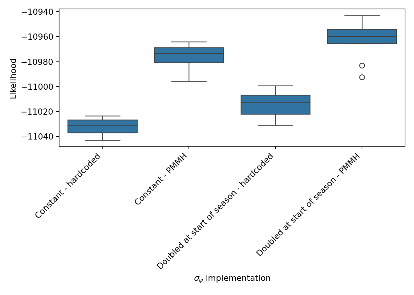

Running the filter online

I’ve looked at the posterior distributions of the filtered states and looked at overall model likelihood, but now I’d like to try and emulate the filter as it would be run in real-time and gain some more useful metrics beyond likelihood (as much as I like likelihoods, sometimes you just want a straight forward accuracy).

The main challenge here is in software, as there isn’t a convenience function for doing this in particles itself. Instead, I looked at the source code to identify how we can step through the updates with each new datapoint. It’s relatively straight forward, just a bit awkward. The filter has its data stored in the data attribute as an an array of $t = 1,\ldots,T$ values, since it assumes that the filter is being run at the end of the time-series at $T$, rather than being run recursively at each $t$. The filter keeps track of its current timepoint in attribute t and at each call of the __next__ method, the filter indexes data by t to get the corresponding data point for its update. This works fine when run offline as all the data up to $T$ is available, but when running offline we only have data available up to the current timepoint $t$.

We’ll need to modify either the t or data attribute to update the filter online then. I’m wary of modifying t since this might have knock on effects elsewhere; data is only used to calculate the likelihood so it seems safer to modify. In essence, t always needs to index into data to obtain the required data. We can achieve this by setting dummy entries for $j=0, 1, \ldots, t-1$ as these values aren’t needed once their likelihood has been calculated.

Show the code


def iterate_dataset(df, mod):
    df = df.copy()
    filt = particles.SMC(
        fk=ssm.Bootstrap(
            mod,
            data=df[['home_score', 'away_score']].values
        ),
        N=1000,
        collect=[Moments()]
    )
    df['home_pred'] = 0.0
    df['draw_pred'] = 0.0
    df['away_pred'] = 0.0
    home_pred_col = np.where(df.columns == 'home_pred')[0][0]
    draw_pred_col = np.where(df.columns == 'draw_pred')[0][0]
    away_pred_col = np.where(df.columns == 'away_pred')[0][0]
    for i, row_raw in enumerate(df.iterrows()):
        dummy, row = row_raw
        if i > 0:
            # Get predictions
            home_id = row['home_id'].astype("int")
            away_id = row['away_id'].astype("int")
            lp_home = np.exp(
                filt.fk.ssm.home_intercept + filt.X[:, home_id] - filt.X[:, away_id]
            )
            lp_away = np.exp(
                filt.fk.ssm.away_intercept + filt.X[:, away_id] - filt.X[:, home_id]
            )
            pred_home = poisson.rvs(lp_home)
            pred_away = poisson.rvs(lp_away)
            df.iloc[i, home_pred_col] = np.mean(pred_home > pred_away)
            df.iloc[i, draw_pred_col] = np.mean(pred_home == pred_away)
            df.iloc[i, away_pred_col] = np.mean(pred_home < pred_away)
        
        # Pass datapoint to model. We can't pass it directly,
        # instead the model seems to work by keep an internal counter
        # its row index in its .data object. So we need to pad out the current
        # datapoint with (i-1) dummy history rows. Slightly awkward as it means we
        # need to keep track of the index too.
        data_point = np.array([[row['home_score'], row['away_score']]])
        if i >= 1:
            padding = np.repeat(np.array([[0, 0]]), i, axis=0)
            data_point = np.concatenate((padding, data_point))
        filt.fk.data = data_point
        
        # Update state
        next(filt)
    return df

Show the code


rps <- function(away_prob, draw_prob, home_prob, outcome) {
    outcome_bools = rep(0, 3)
    outcome_bools[match(outcome, c('away', 'draw', 'home'))] <- 1
    probs <- c(away_prob, draw_prob, home_prob)
    
    0.5 * sum((cumsum(probs) - cumsum(outcome_bools))**2)
}

Show the code


season_res_static_hardcoded = iterate_dataset(
    df[['matchid', 'home_id', 'away_id', 'home_score', 'away_score']], 
    mod1
)
season_res_static_pmmh = iterate_dataset(
    df[['matchid', 'home_id', 'away_id', 'home_score', 'away_score']],
    mod2
)
season_res_double_hardcoded = iterate_dataset(
    df[['matchid', 'home_id', 'away_id', 'home_score', 'away_score']], 
    mod3
)
season_res_double_pmmh = iterate_dataset(
    df[['matchid', 'home_id', 'away_id', 'home_score', 'away_score']], 
    mod4
)

I’ve evaluated all 4 of the candidate models above on 2 metrics: accuracy and RPS, after allowing 3 seasons for the ratings to settle. Reassuringly, these values align with the likelihood scores shown in Figure 8 whereby the model where the variance is doubled at the start of the season using $\sigma_\psi$ estimated using PMMH is the best by RPS (although not accuracy).

NB: the previous sentence is no longer true, as the Static PMMH model is now the best. This is because I reran the filter after writing the text, and the results were quite different. This isn’t a huge surprise as of the 10 runs from the likelihood comparison, 2 of the values from the Double PMMH filter were worse than the median Static PMMH run. I’ve left the original text in as an illustration of the variance between runs, which is something that makes me a bit wary.

Show the code


rbind(
    py$season_res_static_hardcoded |> mutate(alg="Static hardcoded"),
    py$season_res_static_pmmh |> mutate(alg="Static PMMH"),
    py$season_res_double_hardcoded |> mutate(alg="Double hardcoded"),
    py$season_res_double_pmmh |> mutate(alg="Double PMMH")
) |>
    inner_join(py$df |> select(matchid, result, date), by="matchid") |>
    mutate(date = as_date(unlist(date))) |>
    filter(date >= as_date('2008-08-01')) |>
    rowwise() |>
    mutate(
        pred_outcome = c('away', 'draw', 'home')[which.max(c(away_pred, draw_pred, home_pred))]
    ) |>
    ungroup() |>
    rowwise() |>
    mutate(
        rps = rps(away_pred, draw_pred, home_pred, result)
    ) |>
    ungroup() |>
    group_by(alg) |>
    summarise(
        accuracy = mean(result == pred_outcome)*100,
        mean_rps = mean(rps)
    ) |>
    kable("html", col.names = c("Filter", "Accuracy (%)", "Mean RPS"), digits=c(1, 1, 4), align = c("l", "c", "c")) |>
    kable_styling(c("striped", "hover"), full_width=FALSE)

Filter	Accuracy (%)	Mean RPS
Double PMMH	53.5	0.1967
Double hardcoded	52.9	0.2000
Static PMMH	53.7	0.1962
Static hardcoded	53.4	0.1998

Ordinal Logistic Regression

Now that I’ve got some familiarity with particles, I’d like to try the other outcome we’ve modelled previously - match results as an ordinal logistic regression. This is made more complicated by the fact there isn’t such a distribution implementation in the particles package so we need to make one ourselves.

Defining an ordinal logistic distribution

The docs show that a distribution (ProbDist) is defined as having 3 methods:

logpdf: the density function
rvs: drawing a random sample
ppf: the inverse cumulative density function

However, for a basic particle filter only the first is actually needed. An ordinal cumulative distribution function is simply a categorical distribution using probabilities obtained from the linear predictor and the cutpoints $\kappa$, so once we generate probabilities we can just use a standard categorical density.

particles requires a parameterisation such that the outcome x and the cut-points $\kappa$ are constant but the intercept $\phi$ will be a vector of values corresponding to each particle (as $\phi$ depends upon the latent states $\psi$ which varies across particles). The density function for the ordinal logistic distribution is implemented in dordlogit below, which generates the probabilities first and then calls the standard categorical density (dcat_log) function, which is log-transformed as particles works with log-likelihoods. The test output shows that for an outcome of 3 (home win) the density is much higher when the home side is better ($\phi=1$) than when the two teams are equal ($\phi=0$).

Show the code


def dcat_log(prob, outcome):
    return np.log(prob)*outcome + np.log(1-prob)*(1-outcome)

def dordlogit(x, phi, intercepts):
    # X is scalar
    # Phi is N_particles
    # intercepts is 2 (N-outcomes - 1)
    N_particles = phi.size
    n_outcomes = intercepts.size + 1
    intercepts = np.repeat(np.array([intercepts]), N_particles, axis=0)
    q = inv_logit(intercepts - phi.reshape((N_particles, 1)))
    probs = np.zeros((N_particles, n_outcomes))
    probs[:, 0] = q[:, 0]
    for i in range(1, n_outcomes-1):
        probs[:, i] = q[:, i] - q[:, i-1]
    probs[:, n_outcomes-1] = 1-q[:, n_outcomes-2]
    return dcat_log(probs[:, x-1], 1)

np.exp(dordlogit(3, np.array([0, 1]), np.array([np.log(0.2), np.log(0.3)])))

array([0.76923077, 0.9006057 ])

This is ready to be used in a ProbDist, again we’ll leave rvs and ppf blank as they aren’t required for a straight forward bootstrap filter.

Show the code


class OrdLogit(particles.distributions.ProbDist):
    def __init__(self, phi, kappa1, kappa2):
        self.phi = phi
        self.kappa = np.array([kappa1, kappa2])
        
    def logpdf(self, x):
        return dordlogit(x[0], self.phi, self.kappa)
    
    def rvs(self, size=None):
        pass
    
    def ppf(self, u):
        pass

And this distribution is now ready to be used in a StateSpaceModel to predict match outcomes. I’ve used the PoissonModelDoubleVariance model as a template, since it scored the highest; PX0 and PX are identical to before, the only difference is in the likelihood PY. Again, I really appreciate the terseness and declarative nature of the particles classes - so much complexity and behavioural changes are abstracted behind very minor code differences.

Show the code


global home_ids
global away_ids
home_ids = r.df2['home_id'].values
away_ids = r.df2['away_id'].values

class OrdinalModel(ssm.StateSpaceModel):
    def PX0(self):
        return dists.IndepProd(
            *[dists.Dirac(loc=0) for _ in range(N_teams)]
        )
        
    def PX(self, t, xp):
        distributions = [
            get_team_PX(
                xp[:, i],
                t,
                i,
                self.skill_walk_variance
            )
            for i in range(N_teams)
        ]
        return dists.IndepProd(*distributions)
    
    def PY(self, t, xp, x):
        lp = x[:, home_ids[t]] - x[:, away_ids[t]]
        return OrdLogit(phi=lp, kappa1=self.kappa1, kappa2=self.kappa2)

Hardcoded parameters

I’ll now run the filter with some hardcoded parameters, namely using $\sigma_\psi$ that was found to be effective in the Poisson model and values of $\kappa$ that correspond to home and away win probabilities of 50% and 27% respectively, which fortunately convert to nice round log numbers of -1 and 0!

Show the code


mod5 = OrdinalModel(
    kappa1 = -1,
    kappa2 = 0,
    skill_walk_variance=0.017
)
filt5 = particles.SMC(
    fk=ssm.Bootstrap(ssm=mod5, data=r.df2[['result_int']].values),
    N=1000,
    collect=[Moments()]
)
a = time()
filt5.run()
b = time()

# Save final ratings
scores = df[['home', 'home_id']].drop_duplicates().sort_values('home_id')
scores['score'] =  filt5.summaries.moments[df.shape[0]-1]['mean']

print(f"Time taken: {b-a}s")

Time taken: 3.301708221435547s

The resultant ratings are shown in Figure 9 and nowe we can see that Chelsea are definitely ranked the highest, which makes sense as they actually won the league. The rating updates also seem to be far smoother under this Ordinal model despite using the same $\sigma_\psi$ (compare to Figure 1). These two differences are likely because we’re now modelling match outcomes directly rather than identifying which teams are best at scoring goals (which doesn’t always correlate to winning matches), and also because the scale of the linear predictor is different between the two distributions.

Show the code


scores5 <- map_dfr(py$filt5$summaries$moments, function(x) {
    x |> 
        as_tibble() |>
        mutate(teamid = row_number()-1)
}) |>
    mutate(date = rep(df |> filter(league == 'premiership', dset == 'training') |> pull(date), each=py$N_teams)) |>
    inner_join(
        py$df |>
            distinct(home, home_id),
        by=c("teamid"="home_id")
    )

plt_df <- scores5 |>
    filter(date >= as_date('2005-09-01')) |>
    inner_join(teams_all_seasons)

lab_df <- plt_df |>
    group_by(home) |>
    filter(date == max(date)) |>
    summarise(
        date = mean(date),
        mean = mean(mean)
    ) |>
    ungroup()

plt_df |>
    ggplot() +
        geom_rect(aes(xmin=start, xmax=end), ymin=-Inf, ymax=Inf,
                  data=seasons, fill='lightblue', alpha=0.3) +
        geom_line(aes(x=date, y=mean, colour=home)) +
        theme_minimal() +
        geom_label_repel(aes(x=date, y=mean, colour=home, label=home), hjust=0, data=lab_df,
                         max.overlaps = 20) +
        scale_x_datetime(
            expand=expansion(mult=c(0, 0.3)),
            breaks=seq.POSIXt(
                from=as_datetime("2006-01-01"),
                to=as_datetime("2015-01-01"),
                by="1 year"
            ),
            labels=c(
                "2005-2006",
                "2006-2007",
                "2007-2008",
                "2008-2009",
                "2009-2010",
                "2010-2011",
                "2011-2012",
                "2012-2013",
                "2013-2014",
                "2014-2015"
            )
        ) +
        guides(colour="none") +
        theme(
            legend.position = "bottom"
        ) +
        labs(x="", y=TeX("Modelled skill $\\psi$"))

$Change in ratings $\psi$ over time estimated by the Ordinal filter$

Figure 9: Change in ratings $\psi$ over time estimated by the Ordinal filter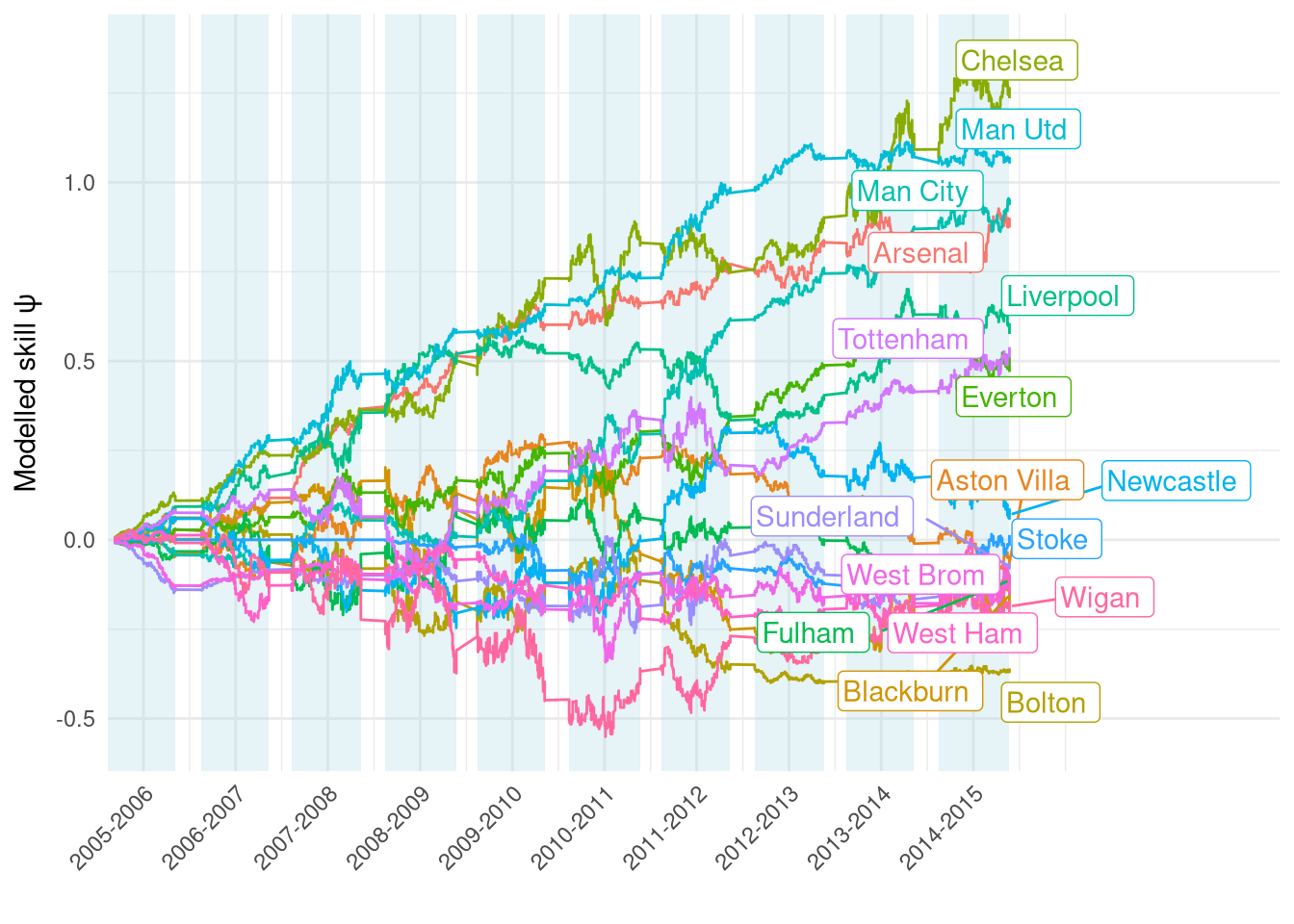

Parameters estimated using PMMH

I also used PMMH to estimate the parameters again, using uninformative priors on both $\sigma_\psi$ and $\kappa$.

Show the code


prior_dict_2 = {
    'skill_walk_variance': dists.LogNormal(mu=0, sigma=1),
    'kappa1': dists.Normal(),
    'kappa2': dists.Normal()
}
prior_2 = dists.StructDist(prior_dict_2)
pmmh_2 = mcmc.PMMH(
    ssm_cls=OrdinalModel,
    prior=prior_2,
    data=df[['result_int']].values,
    Nx=200,     # N particles
    niter=1000  # MCMC iterations
)
a = time()
pmmh_2.run(); 
b = time()
pmmh_2_df = pd.DataFrame(pmmh_2.chain.theta)

Figure 10 shows the resulting traces which are again constant. The intercepts are sensible giving average probabilities of 50% home win, 23% draw, and 27% away win. $\sigma_\psi$ meanwhile is far higher than for the Poisson model at 0.055 vs 0.017, so presumably the ratings will now be much jumpier and more in-line with the Poisson ones.

Show the code


inv_logit <- function(x) 1 / (1 + exp(-x))
py$pmmh_2_df |>
    mutate(sample = row_number()) |>
    filter(sample > 250) |> # Burnin
    mutate(
        kappa1 = inv_logit(kappa1),
        kappa2 = inv_logit(kappa2),
        away = kappa1,
        draw = kappa2 - kappa1,
        home = 1 - kappa2
    ) |>
    select(sample, away, draw, home, skill_walk_variance) |>
    pivot_longer(-sample) |>
    mutate(
        name = factor(
            name, 
            levels=c("home", "draw", "away", "skill_walk_variance"),
            labels=c(TeX("Home win ($1 - \\kappa_2$)"), TeX("Draw ($\\kappa_2 - \\kappa_1$)"), TeX("Away win ($\\kappa_1$)"), TeX("$\\sigma_\\psi$"))
        )
    ) |>
    ggplot(aes(x=sample, y=value)) +
        geom_line() +
        facet_wrap(~name, scales="free", labeller=label_parsed) +
        theme_minimal() +
        labs(x="Sample", y="Value")

Figure 10: PMMH traces from the Ordinal model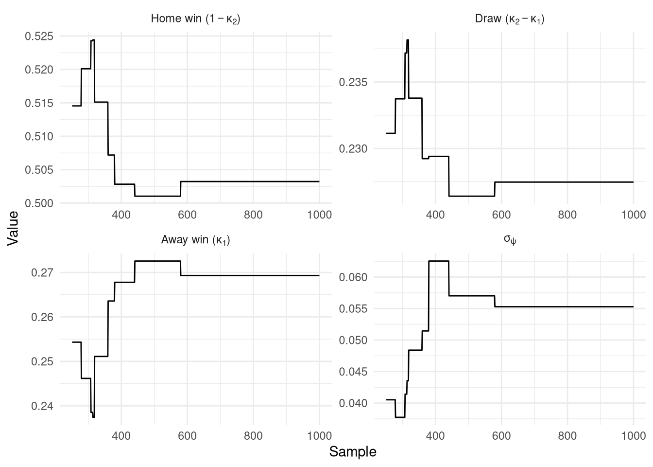

Show the code


mod6 = OrdinalModel(
    kappa1 = np.median(np.array([x[0] for x in pmmh_2.chain.theta])),
    kappa2 = np.median(np.array([x[1] for x in pmmh_2.chain.theta])),
    skill_walk_variance=0.05528829
)
filt6 = particles.SMC(
    fk=ssm.Bootstrap(
        ssm=mod6,
        data=r.df2[['result_int']].values
    ),
    N=1000,
    collect=[Moments()]
)
a = time()
filt6.run()
b = time()

# Save final ratings
scores = df[['home', 'home_id']].drop_duplicates().sort_values('home_id')
scores['score'] =  filt6.summaries.moments[df.shape[0]-1]['mean']

print(f"Time taken: {b-a}s")

Unsurprisingly, the model that uses parameters estimated by PMMH has a much higher likelihood than the hardcoded one (Figure 11) so that will be the ordinal model to compare to the best Poisson model.

Show the code


res_hardcoded = particles.multiSMC(
    fk=ssm.Bootstrap(
        ssm=mod5,
        data=r.df2[['result_int']].values
    ),
    N=1000,
    nruns=10
)
res_auto = particles.multiSMC(
    fk=ssm.Bootstrap(
        ssm=mod6,
        data=r.df2[['result_int']].values
    ),
    N=1000,
    nruns=10
)
res_df = pd.DataFrame({
    'res': 
        [r['output'].logLt for r in res_hardcoded] +
        [r['output'].logLt for r in res_auto],
    'group': 
        ['Hardcoded']*10 +
        ['PMMH']*10
})
plt.clf()
ax = sb.boxplot(res_df, x='group', y='res')
ax.set(xlabel='', ylabel='Likelihood')
ax.set_xticks(ax.get_xticks(), ax.get_xticklabels(), rotation=45, ha='right')
plt.tight_layout()
plt.show()

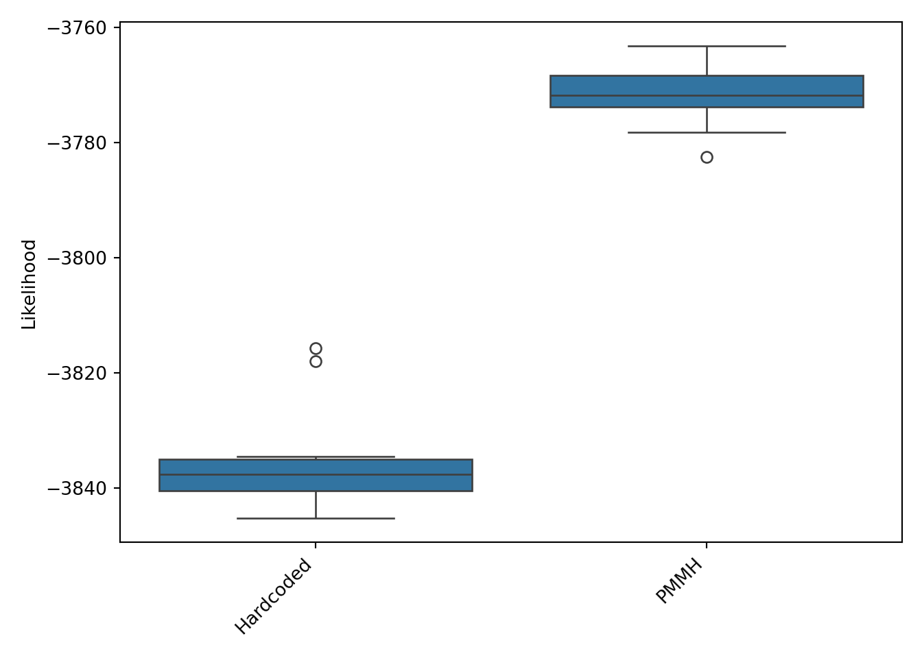
Figure 11: Likelihood comparison of the two Ordinal filters: using a hardcoded set of parameters vs values estimated by PMMH

Figure 12 shows the ratings across the last season for both the Poisson and Ordinal models, demonstrating that there is a far greater varience in $\psi$ in the Ordinal model than in the Poisson. This was also observed in the hierarchical regression, where I speculated it’s due to the fact that the linear predictors are on different scales in both models. I.e. the mean home goals when the 2 teams are equally skilled ($\psi_\text{home} - \psi_\text{away} = 0$) is 1.44, but when the home team is better by 0.5 ($\psi_\text{home} - \psi_\text{away} = 0.5$) the mean goes up to 2.4, quite a large change! However, in the ordinal model the corresponding change in home win probability is “only” from 0.50 to 0.63 (see code chunk below for working). Despite this difference in scale, and the higher $\sigma_\psi$, the ratings generated by the Ordinal filter look very smooth in their updating.

This plot also highlights yet again the large difference between filter runs due to the parameter values and just run-to-run variance, as with these PMMH estimatd parameters Chelsea are now by far the best team and it’s even got Arsenal in second, far ahead of Man City. This is very different to the ratings under $\sigma_\psi=0.01$ in Figure 9.

Show the code


# calculate difference in lambda for a 0.5 change in psi from poisson filter
lambda_0 = np.exp(filt4.fk.ssm.home_intercept)
lambda_1 = np.exp(filt4.fk.ssm.home_intercept + 0.5)

# likewise change in win probabilities for 0.5 change in psi from ordinal filter
intercepts = np.array([filt6.fk.ssm.kappa1, filt6.fk.ssm.kappa2])
q0 = np.concatenate(([0], inv_logit(intercepts), [1]))
probs0 = np.diff(q0)
q1 = np.concatenate(([0], inv_logit(intercepts-0.5), [1]))
probs1 = np.diff(q1)

Show the code


scores4 <- map_dfr(py$filt4$summaries$moments, function(x) {
    x |> 
        as_tibble() |>
        mutate(teamid = row_number()-1)
}) |>
    mutate(date = rep(df2 |> pull(date), each=py$N_teams)) |>
    inner_join(
        df2 |>
            distinct(home, home_id),
        by=c("teamid"="home_id")
    ) |>
    mutate(date = as_date(unlist(date)))

scores6 <- map_dfr(py$filt6$summaries$moments, function(x) {
    x |> 
        as_tibble() |>
        mutate(teamid = row_number()-1)
}) |>
    mutate(date = rep(df |> filter(league == 'premiership', dset == 'training') |> pull(date), each=py$N_teams)) |>
    inner_join(
        py$df |>
            distinct(home, home_id),
        by=c("teamid"="home_id")
    )

teams_last_season <- df |>
    filter(season == '2014-2015') |>
    distinct(home)
    
plt_df <- scores4 |>
    filter(date >= '2014-08-01') |>
    mutate(model="Poisson") |>
    rbind(
        scores6 |>
            filter(date >= '2014-08-01') |>
            mutate(model="Ordinal") 
    ) |>
    inner_join(teams_last_season)

lab_df <- plt_df |>
    group_by(home, model) |>
    filter(date == max(date)) |>
    summarise(
        date = mean(date),
        mean = mean(mean)
    ) |>
    ungroup()

plt_df |>
    mutate(
        model = factor(model, levels=c("Poisson", "Ordinal")) 
    ) |>
    ggplot() +
        geom_line(aes(x=date, y=mean, colour=home)) +
        theme_minimal() +
        facet_wrap(~model) +
        geom_label_repel(aes(x=date, y=mean, colour=home, label=home), hjust=0, data=lab_df,
                         max.overlaps = 20) +
        scale_x_datetime(expand=expansion(mult=c(0, 0.3))) +
        guides(colour="none") +
        theme(
            legend.position = "bottom"
        ) +
        labs(x="", y=TeX("Modelled skill $\\psi$"))

$Comparison of $\psi$ estimated by the two Ordinal filters$

Figure 12: Comparison of $\psi$ estimated by the two Ordinal filters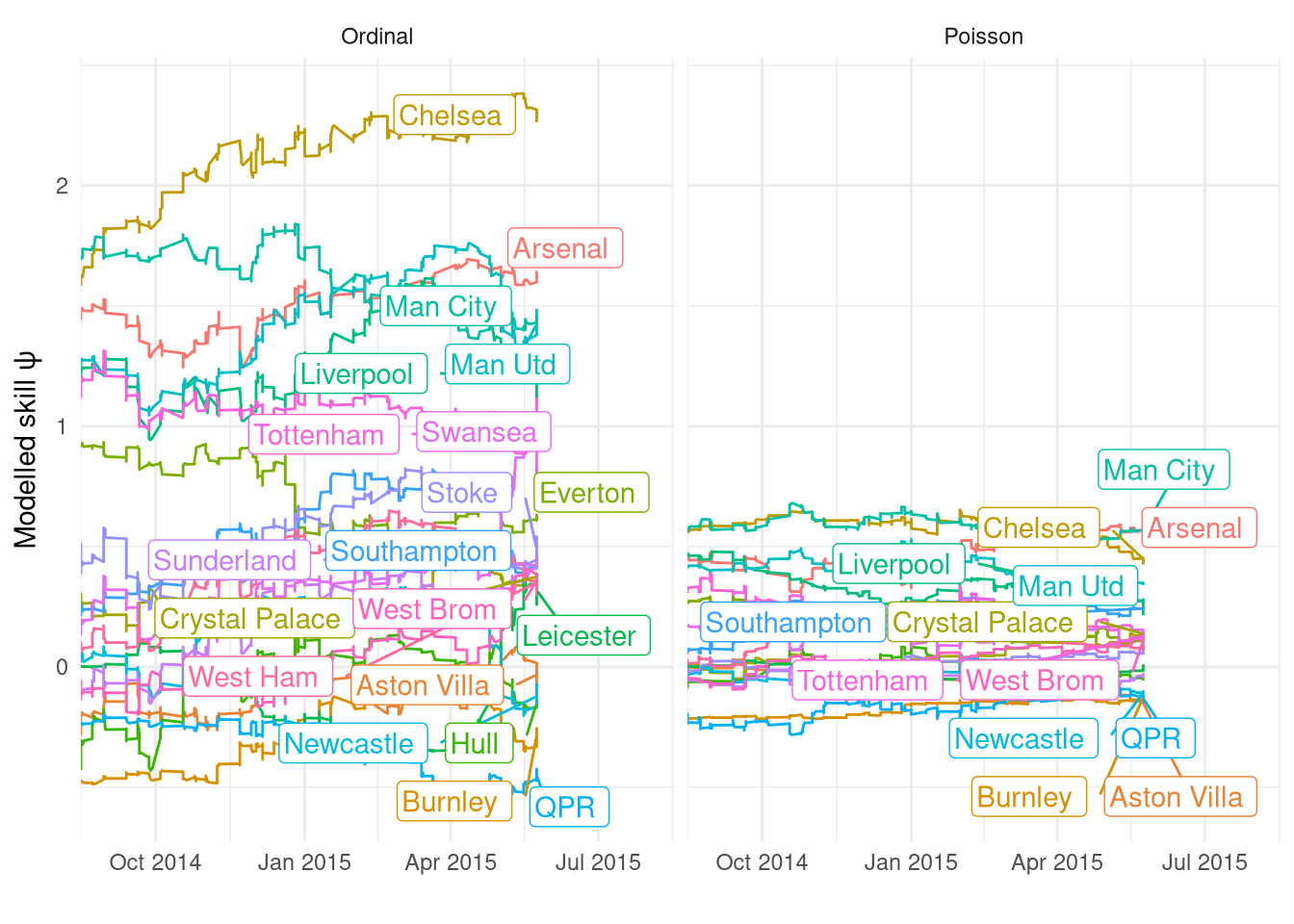

For the final comparison I’ve run the Ordinal model (with the PMMH estimated parameters) through the entire training set in online mode and compared its metrics to the Poisson filter. I’ve also added an extra metric for evaluation: the mean absolute difference in the final ranking compared to the actual league position so as to provide another facet of comparison rather than just match prediction accuracy.

Surprisingly, both models have the exact same accuracy to 3 digits! In terms of RPS and ranking error there is a split: the Poisson model is favoured by RPS and the Ordinal model is very slightly better at the rating (which makes sense as the Ordinal filter forms its skill based on match ratings just like the actual standings). Therefore it might be the case that both models are needed to provide a full picture: the Poisson model is better at predicting match outcomes, but the Ordinal model’s rating is closer to their actual league standing.

Show the code


rng = np.random.default_rng()
def iterate_dataset_ordinal(df, mod):
    df = df.copy()
    filt = particles.SMC(
        fk=ssm.Bootstrap(
            mod,
            data=df[['result_int']].values
        ),
        N=1000,
        collect=[Moments()]
    )
    N_particles = 1000
    N_outcomes = 3
    df['home_pred'] = 0.0
    df['draw_pred'] = 0.0
    df['away_pred'] = 0.0
    home_pred_col = np.where(df.columns == 'home_pred')[0][0]
    draw_pred_col = np.where(df.columns == 'draw_pred')[0][0]
    away_pred_col = np.where(df.columns == 'away_pred')[0][0]
    for i, row_raw in enumerate(df.iterrows()):
        dummy, row = row_raw
        if i > 0:
            # Get predictions
            home_id = row['home_id'].astype("int")
            away_id = row['away_id'].astype("int")
            phi = filt.X[:, home_id] - filt.X[:, away_id]
            intercepts = np.array([filt.fk.ssm.kappa1, filt.fk.ssm.kappa2])
            
            # Form probabilities
            q = inv_logit(intercepts - phi.reshape((N_particles, 1)))
            probs = np.zeros((N_particles, N_outcomes))
            probs[:, 0] = q[:, 0]
            for k in range(1, N_outcomes-1):
                probs[:, k] = q[:, k] - q[:, k-1]
            probs[:, N_outcomes-1] = 1-q[:, N_outcomes-2]
            
            # Draw posterior predictive outcomes from multinomial
            draws = rng.multinomial(1, probs)
            
            # Derive probabilities of each outcome and save
            predictive_probs = draws.sum(axis=0) / N_particles
            df.iloc[i, away_pred_col] = predictive_probs[0]
            df.iloc[i, draw_pred_col] = predictive_probs[1]
            df.iloc[i, home_pred_col] = predictive_probs[2]
        
        # Pass datapoint to model
        data_point = np.array([[row['result_int']]]).astype("int")
        if i >= 1:
            padding = np.repeat(np.array([[0]]), i, axis=0)
            data_point = np.concatenate((padding, data_point))
            
        filt.fk.data = data_point
        
        # Update state
        next(filt)
    return df

Show the code


season_res_ordinal = iterate_dataset_ordinal(
    r.df2[['matchid', 'home_id', 'away_id', 'result_int']],
    mod6
)

Show the code


rating_mae <- scores4 |>
    mutate(model = 'Poisson') |>
    rbind(
        scores6 |> mutate(model = 'Ordinal')
    ) |>
    group_by(model, home) |> 
    filter(date == max(date)) |> 
    ungroup() |>
    group_by(model, home) |>
    summarise(score = median(mean)) |>
    ungroup() |> 
    rename(team=home) |>
    group_by(model) |>
    mutate(
        rating_rank = rank(-score),
    ) |>
    inner_join(
        league_positions_training, by="team"
    ) |>
    mutate(
        difference = position - rating_rank
    ) |>
    group_by(model) |>
    summarise(
        mae = mean(abs(difference))
    )

rbind(
    py$season_res_ordinal |> 
        select(matchid, home_pred, draw_pred, away_pred) |>
        mutate(model="Ordinal"),
    py$season_res_double_pmmh |> 
        select(matchid, home_pred, draw_pred, away_pred) |>
        mutate(model="Poisson")
) |>
    inner_join(py$df |> select(matchid, result, date), by="matchid") |>
    mutate(date = as_date(unlist(date))) |>
    filter(date >= as_date('2008-08-01')) |>
    rowwise() |>
    mutate(
        pred_outcome = c('away', 'draw', 'home')[which.max(c(away_pred, draw_pred, home_pred))]
    ) |>
    ungroup() |>
    rowwise() |>
    mutate(
        rps = rps(away_pred, draw_pred, home_pred, result)
    ) |>
    ungroup() |>
    group_by(model) |>
    summarise(
        accuracy = mean(result == pred_outcome)*100,
        mean_rps = mean(rps)
    ) |>
    inner_join(rating_mae, by="model") |>
    select(model, accuracy, mean_rps, mae) |>
    kable("html", col.names = c("Filter", "Accuracy (%)", "Mean RPS", "Mean ranking error"), digits=c(1, 1, 4, 3), align = c("l", "c", "c", "c")) |>
    kable_styling(c("striped", "hover"), full_width=FALSE)

Filter	Accuracy (%)	Mean RPS	Mean ranking error
Ordinal	53.5	0.1991	2.9
Poisson	53.5	0.1967	3.1

Conclusion

However, if I were to use one of these filters in production, I’d definitely want to sort out some of the niggles mentioned throughout this post: the fact that ratings are updated for teams that didn’t play, PMMH having minimal variance, and the not-insignificant inter-run variance. I will likely need to use a more bespoke model rather than the SSM wrapper that particles provide, and will probably need to investigate filters beyond the basic Bootstrap filter that I’ve been using thus far.

Hopefully once I’ve finished the book I’ll have the knowledge to develop a more bespoke model that addresses these concerns. Until then, I’ll use these two filters in the next (and final!) post in this series, where the final comparison on all the models introduced in these four parts will be undertaken on the as-yet-unseen test set. Stay tuned.

Predictaball retrospective part 4 - Particle Filters

Introduction

Particle Filters

Setup

Poisson model of goals scored

Bayesian parameter inference - PMMH

Increasing skill variance at the start of the season

Running the filter online

Ordinal Logistic Regression

Defining an ordinal logistic distribution

Hardcoded parameters

Parameters estimated using PMMH

Conclusion

Related