Introduction
Following on from Part 1 in this series of posts looking back at the history of Predictaball, I’ll be reexamining the Elo models that were used from 2017-2019. One obvious flaw with the hierarchical Bayesian regression model was that there was no acknowledgement of time - a team’s skill was modelled at the point of training and kept fixed from them on. The model could be retrained after each match, but MCMC is time-consuming, and the resultant skill would still be an average over the full training period rather than the value at the current time. In my professional work I was also working more closely with prognostic indices of health, which use very simple hand-crafted equations to provide an estimate of disease severity. While they contain far less information than a data-driven model, they are cheap to run (both in the sense of not needing any training but also at prediction time), and are very interpretable by design.
I was therefore interested to try using standard Elo models on Predictaball as these would share much of the same benefits as the prognostic indices, as well as taking the temporal dimension into account.
Show the code
library(tidyverse)
library(knitr)        # Displaying tables
library(kableExtra)   # Displaying tables
library(ggrepel)      # Plotting
library(ggridges)     # Plotting
library(latex2exp)    # Math-mode in plots
library(patchwork)    # Combining plots
options(knitr.table.html.attr = "quarto-disable-processing=true")
Elo model
I have full details of the Elo model in a previous post, but I’ll quickly summarise it here. Elo rating systems have 2 components (notice the similarity to state-space models both here and later on):
- A prediction step that predicts the result for a given match given the rating difference between the teams
- An update step that uses the predicted result and the actual outcome to determine how much to update both teams’ rating by
Both of these parts are typically hand-crafted with generally human interpretable values.
Prediction step
Elo systems are defined for binary outcomes and therefore output a scalar value in $[0, 1]$, where 0 means team 1 loses / team 2 wins, and 1 means a team 1 victory / team 2 loss. This can be considered analogous to the probability parameter of a Binomial distribution. They can be extended to multiple outputs, such as in football where a draw is possible, by assigning 0.5 to a draw.
The equation used in this football rating system uses a logistic function just like the Binomial distribution to map the difference in the teams’ ratings into $[0, 1]$, although unlike the binomial it uses base 10 rather than the natural log. The dividing by 400 just scales the rating difference (which can be in the order of magnitude of hundreds, as the starting rating is 1000).
$$E = \frac{1}{1 + 10^{-(\psi_\text{home} - \psi_\text{away}) / 400}}$$
Result predictions against rating differences are shown in Figure 1, with the characteristic sigmoid S-curve appearing. The plot also highlights the limited information that his model provides in comparison to last post’s Bayesian regression models, where a full distribution is available for the output prediction allowing for the use of probabilistic statements. If the sport was truly binary then this rating could be used as the input to a Binomial distribution, but instead for football we are stuck with just a scalar prediction.
Show the code
E <- function(delta) {
    1 / (1 + 10**(-delta / 400))
}

tibble(
    skill_difference = -1000:1000,
    prob_home = E(skill_difference)
) |>
    ggplot(aes(x=skill_difference, y=prob_home)) +
        geom_hline(yintercept=0, linetype="dashed", colour="lightsalmon") +
        geom_hline(yintercept=0.5, linetype="dashed", colour="forestgreen") +
        geom_hline(yintercept=1, linetype="dashed", colour="lightblue") +
        annotate("label", x=-Inf, y=1, label="Home win", colour="lightblue", hjust=0) +
        annotate("label", x=-Inf, y=0.5, label="Draw", colour="forestgreen", hjust=0) +
        annotate("label", x=-Inf, y=0, label="Away win", colour="lightsalmon", hjust=0) +
        geom_line() +
        theme_minimal() +
        labs(
            x=TeX("$\\psi_{home} - \\psi_{away}$"),
            y="E"
        )
Figure 1: Match prediction in Elo model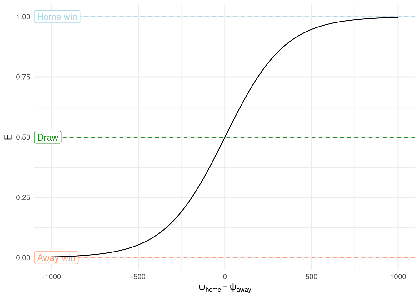
The plot also shows that the prediction is symmetrical around 0, however, as seen last time (and will be immediately obvious to anyone with a passing interest in football), the home team has an advantage, and this advantage can also very by league. This is solved in the Elo model by adding an intercept $\alpha$ which represents the number of rating points that the home side is advantaged by. The value of $\alpha$ has been identified manually and set to 64 for the Premiership (68 for La Liga, 67 for Serie A, and 56 for Bundesliga).
$$\eta = \alpha + \psi_\text{home} - \psi_\text{away}$$
$$E = \frac{1}{1 + 10^{-\eta / 400}}$$
Figure 2 shows the expected outcomes with home advantage added in, although the difference between leagues is relatively small when viewed at this scale.
Show the code
tribble(
    ~league, ~HA,
    "Premiership", 64,
    "La Liga", 68,
    "Bundesliga", 56,
    "Serie A", 67
) |>
    expand_grid(
        tibble(
            skill_difference = -1000:1000,
            prob_home = E(skill_difference)
        )
    ) |>
    mutate(
        skill_difference_with_HA = skill_difference+HA,
        prob_home = E(skill_difference_with_HA)
    ) |>
    ggplot(aes(x=skill_difference, y=prob_home, colour=league)) +
        geom_hline(yintercept=0, linetype="dashed", colour="lightsalmon") +
        geom_hline(yintercept=0.5, linetype="dashed", colour="forestgreen") +
        geom_hline(yintercept=1, linetype="dashed", colour="lightblue") +
        annotate("label", x=-Inf, y=1, label="Home win", colour="lightblue", hjust=0) +
        annotate("label", x=-Inf, y=0.5, label="Draw", colour="forestgreen", hjust=0) +
        annotate("label", x=-Inf, y=0, label="Away win", colour="lightsalmon", hjust=0) +
        geom_line() +
        theme_minimal() +
        labs(
            x=TeX("$\\alpha + \\psi_{home} - \\psi_{away}$"),
            y="E"
        ) +
        scale_colour_brewer("", palette="Dark2") +
        theme(
            legend.position = "bottom"
        )
Figure 2: Match prediction with home advantage included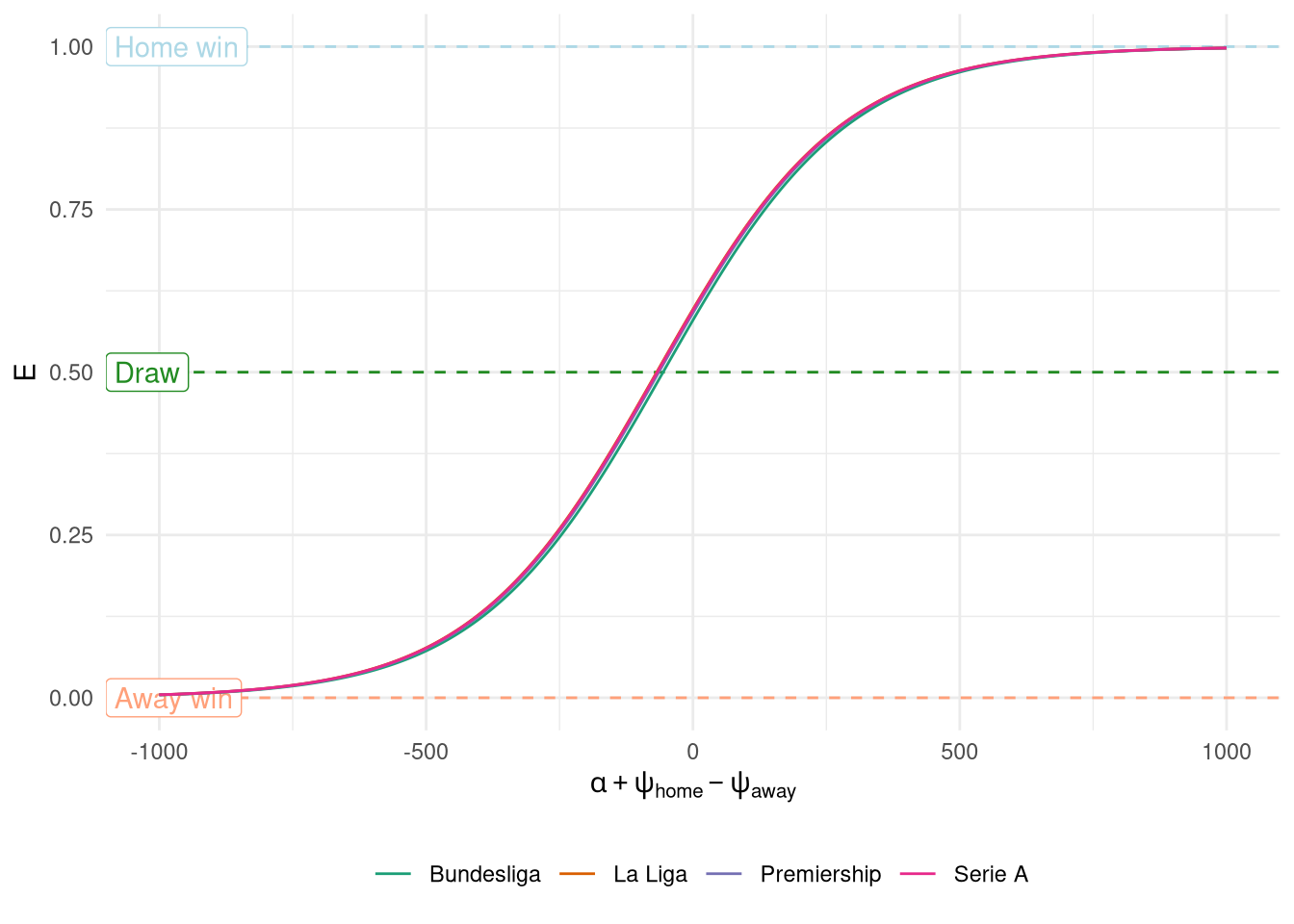
Update step
The next step is to calculate the change in ratings $\delta$ using the difference between the predicted and actual result, multiplied by a gain $K$ (again compare to state-space models). $\delta$ is defined as the rating change for the home team, and because Elo requires a zero-sum game, the away team’s change is defined as $-\delta$.
$$\delta = K(O - E)$$
$K$ controls how much a team’s rating is determined by the previous match (high $K$) vs being a smoother long term average (low $K$), just like $\alpha$ in an Exponential Moving Average filter. For example, in club football where teams play each other regularly you would prefer to keep K lower to focus on the long term trend, whereas in international football where matches are far less frequent it would make sense to use a higher $K$. $K$ was chosen as 20 for Predictaball, so that this is the maximum rating change from one game by inspecting various scenarios with different values of $K$ to find the balance between the rating showing long term trends whilst still responding to recent matches.
One way in which this trade-off can be achieved is by keeping $K$ relatively low, but assigning higher weight to larger victories - as it stands the equation treats a 1-0 win the same as an 8-0 blowout - but in reality the latter demonstrates more skill difference and should result in a higher rating gain.
This was achieved by extending the update equation to take into account the margin of victory via a function $G(x)$.
$$\delta = KG(\Delta)(O - E)$$
$$\Delta = \text{goals}_\text{home} - \text{goals}_\text{away}$$
This function has a log form so there are diminishing returns associated with higher goals being scored (after all the difference between a 6-0 and 7-0 victory is probably less than the difference between a 1-0 and 2-0), as shown in Figure 3.
$$ \displaylines{ G(\Delta) = \begin{cases} 1 & \text{if } \Delta \leq 1 \\ \log_2(1.7\Delta) & \text{otherwise} \end{cases} } $$
Show the code
G_func <- function(MOV) {
    ifelse(MOV <= 1, 1, log2(MOV * 1.7))
}
expand_grid(
    O=c(0, 0.5, 1),
    E=seq(0, 1, length.out=1000),
    K=c(20),
    MOV=seq(0, 8)
) |>
    filter(
        !(MOV > 0 & O == 0.5),
        !(MOV == 0 & O %in% c(0, 1))
    ) |>
    mutate(
        delta = K * G_func(MOV) * (O-E),
        outcome = factor(O, levels=c(1, 0.5, 0), labels=c("Result=Home win", "Result=Draw", "Result=Away win")),
        K_lab = factor(K, levels=c(1, 10, 20, 100), labels=c("K=1", "K=10", "K=20", "K=30")),
        MOV_fact = factor(
            ifelse(MOV <= 1, '0-1', as.character(MOV))
        )
    ) |>
    ggplot(aes(x=E, y=delta)) +
        geom_rect(xmin=-Inf, xmax=Inf, ymin=0, ymax=Inf, fill='lightblue', alpha=0.1) +
        geom_rect(xmin=-Inf, xmax=Inf, ymin=-Inf, ymax=0, fill='lightsalmon', alpha=0.1) +
        geom_line(aes(colour=MOV_fact)) +
        annotate("label", x=-Inf, y=-Inf, label="Away team wins points", vjust=0, hjust=0) +
        annotate("label", x=Inf, y=Inf, label="Home team wins points", vjust=1, hjust=1) +
        facet_wrap(~outcome, scales="fixed") +
        theme_bw() +
        labs(x="E", y=TeX("Goal difference ($\\delta$)")) +
        scale_colour_viridis_d(TeX("\\Delta")) +
        theme(
            legend.position = "bottom"
        )
Figure 3: Elo rating update $\delta$ as a function of prediction $E$ and margin of victory $\Delta$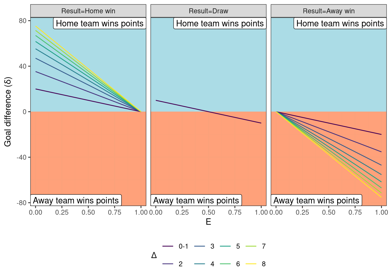
Putting it all together
The code below shows a function that takes a match parameterised by the goals scored by both sides, the pre-match ratings of both teams, the result, and the league, and applies both equations in series to calculate the new ratings.
Show the code
ratings_update_elo <- function(home_score, away_score, home_elo, away_elo, league, result) {
    K <- 20
    HA <- list(
        "premiership"=64,
        "laliga"=68,
        "bundesliga1"=56,
        "seriea"=66
    )[[league]]

    # Calculate E
    dr_home <- (home_elo + HA) - away_elo
    E <- 1 / (1 + 10 ** (-dr_home / 400.0))

    # Calculate G
    MOV <- abs(home_score - away_score)
    G <- G_func(MOV)
    O <- list(
        'away'= 0,
        'draw'= 0.5,
        'home'= 1
    )[[result]]


    # Calculate updates
    update <- K * G * (O - E)

    # Update elos
    new_home = round(home_elo + update)
    new_away = round(away_elo - update)

    c(new_home, new_away, E)
}
We can run a season through this rating system to see how it works in practice, although I’ll stick to a single season to avoid having to make decisions about how to handle relegated/promoted teams. I’ll use the first season of the Premiership in the training data for this purpose, which is 2005-2006.
Show the code
df_2005 <- df |>
    filter(league == 'premiership', season == '2005-2006') |>
    arrange(date) |>
    mutate(
        home_elo = NA_real_,
        away_elo = NA_real_,
        E_pred = NA_real_
    )

teams_2005 <- unique(df_2005$home)
teams_2005 <- setNames(teams_2005, teams_2005)
start_elo <- 1000
elos_current <- lapply(teams_2005, function(x) start_elo)

for (i in 1:nrow(df_2005)) {
    # Save old elos
    df_2005$home_elo[i] <- elos_current[[df_2005$home[i]]]
    df_2005$away_elo[i] <- elos_current[[df_2005$away[i]]]

    # Calculate new elos
    new_elos <- ratings_update_elo(
        df_2005$home_score[i],
        df_2005$away_score[i],
        elos_current[[df_2005$home[i]]],
        elos_current[[df_2005$away[i]]],
        df_2005$league[i],
        df_2005$result[i]
    )

    # Save new elos and E
    elos_current[[df_2005$home[i]]] <- new_elos[1]
    elos_current[[df_2005$away[i]]] <- new_elos[2]
    df_2005$E_pred[i] = new_elos[3]
}
Figure 4 shows how each team’s rating changed from the default starting value of 1000 over the course of the 38 matches. It’s relatively smooth and while individual matches can be identified by little jumps, they don’t dominate or change the trend.
Show the code
# Get last elo from each time
elo_final <- tibble(
    date = max(df_2005$date + days(1)),
    team = names(elos_current),
    elo = unlist(elos_current)
)
# Extract elos from match data frame
df_2005 |>
    select(date, home_team=home, away_team=away, home_elo, away_elo) |>
    pivot_longer(c(home_team, away_team), values_to="team") |>
    mutate(
        elo = ifelse(name == 'home_team', home_elo, away_elo)
    ) |>
    select(date, team, elo) |>
    # Add on last elo
    rbind(
        elo_final
    ) |>
    ggplot(aes(x=date, y=elo, colour=team)) +
        geom_line() +
        geom_label_repel(
            aes(x=date, y=elo, label=team),
            data=elo_final
        ) +
        labs(x="", y=TeX("Elo rating $\\psi$")) +
        guides(colour="none") +
        theme_minimal()
Figure 4: Rating change over 2005-2006 Premiership season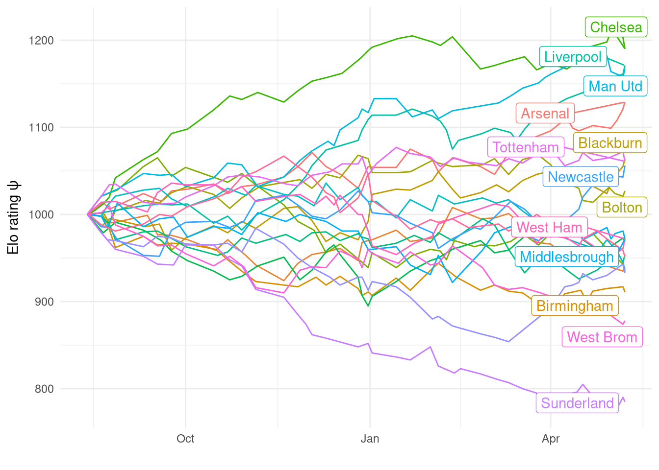
As shown in the table below, the end-of-season ratings for each time correlate very strongly with the final league standings (Spearman correlation = 0.96), which is particularly impressive given that the rating system only had 1 year of data to learn from.
Show the code
standings_2005 <- tribble(
    ~team, ~position,
    "Chelsea", 1,
    "Man Utd", 2,
    "Liverpool", 3,
    "Arsenal", 4,
    "Tottenham", 5,
    "Blackburn", 6,
    "Newcastle", 7,
    "Bolton", 8,
    "West Ham", 9,
    "Wigan", 10,
    "Everton", 11,
    "Fulham", 12,
    "Charlton", 13,
    "Middlesbrough", 14,
    "Man City", 15,
    "Aston Villa", 16,
    "Portsmouth", 17,
    "Birmingham", 18,
    "West Brom", 19,
    "Sunderland", 20
)

tab_df <- standings_2005 |>
    inner_join(
        elo_final,
        by="team"
    ) |>
    mutate(
        rank_elo = rank(-elo),
        rank_diff = abs(position - rank_elo)
    ) |>
    select(team, position, rank_elo, rank_diff)

tab_df |>
    kable("html", col.names = c("Team", "Final league position", "Elo rank", "Difference between ranks"),
          align=c("l", "c", "c", "c")) |>
    kable_styling(c("striped", "hover"), full_width=FALSE)  |>
    column_spec(
        4, color = ifelse(tab_df$rank_diff == 0, 'green', 'red')
    )
| Team | Final league position | Elo rank | Difference between ranks |
|---|---|---|---|
| Chelsea | 1 | 1.0 | 0.0 |
| Man Utd | 2 | 3.0 | 1.0 |
| Liverpool | 3 | 2.0 | 1.0 |
| Arsenal | 4 | 4.0 | 0.0 |
| Tottenham | 5 | 6.0 | 1.0 |
| Blackburn | 6 | 5.0 | 1.0 |
| Newcastle | 7 | 7.0 | 0.0 |
| Bolton | 8 | 8.0 | 0.0 |
| West Ham | 9 | 9.5 | 0.5 |
| Wigan | 10 | 13.0 | 3.0 |
| Everton | 11 | 11.0 | 0.0 |
| Fulham | 12 | 12.0 | 0.0 |
| Charlton | 13 | 16.0 | 3.0 |
| Middlesbrough | 14 | 9.5 | 4.5 |
| Man City | 15 | 15.0 | 0.0 |
| Aston Villa | 16 | 14.0 | 2.0 |
| Portsmouth | 17 | 17.0 | 0.0 |
| Birmingham | 18 | 18.0 | 0.0 |
| West Brom | 19 | 19.0 | 0.0 |
| Sunderland | 20 | 20.0 | 0.0 |
Prediction model - Ordinal
The rating system seems to work quite well - it produces ratings that look sensible and align with the league table and is easily intepretable. However, the ultimate aim is to predict match outcomes, and here Elo falls a little short for football. The prediction $E$ is designed for binary games and doesn’t provide probabilistic predictions for the multinomial output of a football match. Furthermore, as shown in Figure 5, $E$ doesn’t seem particularly well calibrated at all, with it barely changing regardless if the match was a home win or away win.
Show the code
df_2005 |>
    mutate(
        result = factor(
            result,
            levels=c("home", "draw", "away"),
            labels=c("Home win", "Draw", "Away win")
        )
    ) |>
    ggplot(aes(y=result, x=E_pred)) +
        geom_boxplot() +
        theme_minimal() +
        xlim(0, 1) +
        labs(x="E", y="")
Figure 5: Elo match predictions $E$ against actual outcomes for the 2005-2006 Premiership season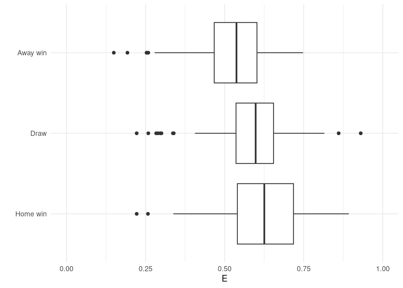
Instead of using $E$ as the overall match prediction, I’ll keep using it to update ratings, but generate a separation prediction model focused on the match prediction task. I’ll use an ordinal logistic regression prediction model for all the same reasons as last time. This particular regression model was used in conjunction with the Elo rating system for the 2017-2018 season but I’ve lost the full model definition and only have the posterior draws saved along with a function for generating posterior predictive draws.
The likelihood is extremely similar to the latent skill model discussed in the last post, but now the skill difference is input data rather than a latent parameter, which means we can scale it by a coefficient $\beta$ as needed without worrying about identifiability. Again the cut-offs $\kappa$ are league-specific. I don’t have the priors saved anywhere but I imagine they are relatively uninformative.
$$\text{result}_i \sim \text{Ordered-logit}(\phi_i,k_i)$$
$$\phi_i = \beta(\psi_\text{home[i]} - \psi_\text{away[i]})$$
$$k_i = \kappa_{\text{league[i]}}$$
The posterior distribution of $\kappa$ is shown in Figure 6, and reinforces the previous finding that Serie A has the lowest proportion of away wins, but we no longer see the Bundesliga as having the highest away win rate - likely because this model was trained on a different dataset.
Show the code
league_ord <- c("bundesliga1", "laliga", "premiership", "seriea")
league_labels <- c("Bundesliga", "La Liga", "Premiership", "Serie A")
inv_logit <- function(x) {
    exp(x) / (1 + exp(x))
}
mod_elo_ordinal$coefs |>
    as_tibble() |>
    select(starts_with("alpha")) |>
    mutate(sample = row_number()) |>
    pivot_longer(
        -sample,
        names_pattern="alpha\\[([1-4]),([1-2])\\]",
        names_to=c("league_id", "intercept_id")
    ) |>
    mutate(
        league_id = as.integer(league_id),
        league = factor(league_id, levels=1:4, labels=mod_elo_ordinal$leagues),
        league = factor(league, levels=league_ord, labels=league_labels),
        value = inv_logit(value)
    ) |>
    select(-league_id) |>
    pivot_wider(names_from = "intercept_id", values_from="value") |>
    mutate(
        `3` = 1 - `2`,
        `2` = `2` - `1`
    ) |>
    pivot_longer(c(`1`, `2`, `3`)) |>
    mutate(
        event = factor(name, levels=c(3, 2, 1), labels=c("Home win", "Draw", "Away win")),
    ) |>
    ggplot(aes(x=value, group=league, fill=league)) +
        geom_density() +
        facet_wrap(~event, ncol=1) +
        theme_minimal() +
        scale_fill_brewer("", palette="Dark2") +
        scale_x_continuous() +
        labs(x=latex2exp::TeX("Probability of event (inv_logit(\\kappa))")) +
        theme(
            legend.position = "bottom"
        )
Figure 6: Posterior $\kappa$ distributions for the ordinal logistic match prediction model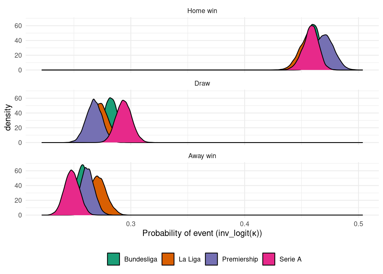
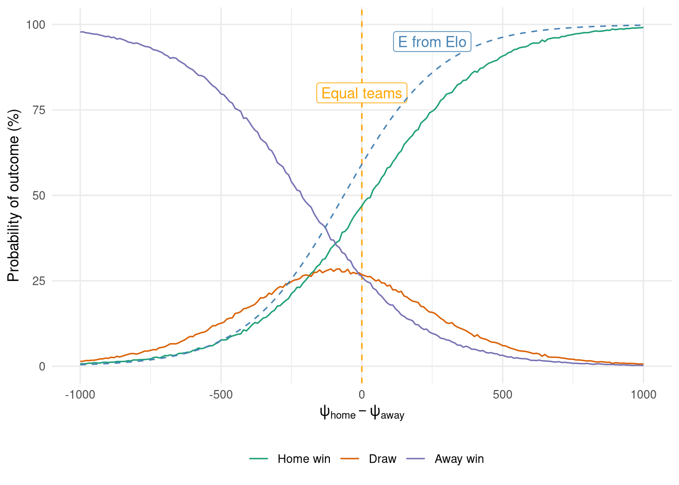
The relationship between the Elo difference between the two teams and the predicted outcome is shown in Figure 7. It shows several things of note, including the home advantage, the interesting fact that a draw is never the most probable outcome, as well the close similarity between the home probability and the expected outcome $E$ from the Elo system. However, it also highlights how much more information is available from the ordinal logistic regression as we get probabilities for draws too, which explains the vertical gap between $E$ prediction and that of a home win from the ordinal model.
Show the code
get_probabilities <- function(phi, kappa) {
    # phi is 1d array
    # kappa is 2d array
    N_samples <- length(phi)
    q <- inv_logit(kappa - phi)
    probs <- matrix(nrow=N_samples, ncol=3)
    probs[, 1] <- q[, 1]
    probs[, 2] <- q[, 2] - q[, 1]
    probs[, 3] <- 1 - q[, 2]
    probs
}

rordlogit_vectorized <- function(phi, kappa) {
    probs <- get_probabilities(phi, kappa)
    cumprobs <- t(apply(probs, 1, cumsum))
    thresh <- runif(nrow(probs))
    apply(cumprobs > thresh, 1, which.max)
}

predict_elo_ordinal <- function(elo_diff, league) {
    coefs <- mod_elo_ordinal$coefs
    league_num <- which(mod_elo_ordinal$leagues == league)

    # Calculate phi
    elo_scale <- (elo_diff - mod_elo_ordinal$elodiff_center) / mod_elo_ordinal$elodiff_scale
    phi <- coefs[, "beta"] * elo_scale

    # Obtain kappa as [N_samples, 2]
    alpha_1_col <- paste0("alpha[", league_num, ",1]")
    alpha_2_col <- paste0("alpha[", league_num, ",2]")
    kappa <- coefs[, c(alpha_1_col, alpha_2_col)]

    draws <- rordlogit_vectorized(phi, kappa)
    preds <- as.numeric(table(draws) / length(draws))
    tibble(away_prob=preds[1], draw_prob=preds[2], home_prob=preds[3])
}
Show the code
elo_diffs <- seq(-1000, 1000, by=10)
map_dfr(elo_diffs, predict_elo_ordinal, "premiership", .id="elo_diff") |>
    mutate(
        elo_diff = as.integer(as.character(factor(as.integer(elo_diff), labels=elo_diffs)))
    ) |>
    pivot_longer(-elo_diff) |>
    mutate(
        value = value * 100,
        name = factor(
            name,
            levels=c("home_prob", "draw_prob", "away_prob", "E"),
            labels=c("Home win", "Draw", "Away win", "E from Elo")
        )
    ) |>
    ggplot(aes(x=elo_diff, y=value)) +
        geom_vline(xintercept=0, linetype="dashed", colour="orange") +
        annotate("label", x=0, y=80, label="Equal teams", colour="orange") +
        geom_line(aes(group=name, colour=name)) +
        geom_line(
            data=tibble(
                elo_diff = elo_diffs,
                value = E(elo_diff+64) * 100
            ),
            linetype="dashed",
            colour="steelblue"
        ) +
        annotate("label", x=250, y=95, label="E from Elo", colour="steelblue") +
        theme_minimal() +
        ylim(0, 100) +
        guides(linetype="none") +
        scale_color_brewer("", palette="Dark2") +
        labs(x=TeX("$\\psi_{home} - \\psi_{away}$"),
             y="Probability of outcome (%)") +
        theme(
            legend.position = "bottom",
            panel.grid.minor.y = element_blank()
        )
Finally, the posterior predictive check is shown in Figure 8 just like in the last post, and indeed it is similarly awkward to interpret! However, it also shows that the predictions don’t seem very well calibrated, just like $E$ in Figure 5, so perhaps I shouldn’t have judged too harshly. One cause could be that the PPC is only being run on data from this first season, which shouldn’t really be used in its entirety as it takes some time for the ratings to settle as shown in Figure 4. Ideally this would be run on the entire training set but a) I don’t know what the entire training set was anymore, and I don’t know how I handled promotion/relegation back then, so we’ll stick with this flawed check.
Show the code
ppc_ordinal <- map_dfr(1:nrow(df_2005), function(i) {
    predict_elo_ordinal(
        df_2005$home_elo[i] - df_2005$away_elo[i],
        df_2005$league[i]
    ) |>
        mutate(
            date = df_2005$date[i],
            home = df_2005$home[i],
            away = df_2005$away[i],
            result = df_2005$result[i]
        )
})
ppc_ordinal |>
    pivot_longer(c(away_prob, draw_prob, home_prob)) |>
    mutate(
        result = factor(result, levels=c('home', 'draw', 'away'), labels=c('Result=Home', 'Result=Draw', 'Result=Away')),
        name = factor(name, levels=c('home_prob', 'draw_prob', 'away_prob'), labels=c('Prediction=Home', 'Prediction=Draw', 'Prediction=Away'))
    ) |>
    ggplot(aes(x=name, y=value, fill=name)) +
        geom_boxplot() +
        facet_wrap(~result) +
        theme_bw() +
        scale_fill_brewer("Modelled outcome", palette="Dark2") +
        labs(x="", y="Posterior predictive probability") +
        guides(fill="none") +
        theme(
            legend.position = "bottom",
            axis.text.x = element_text(angle=45, hjust=1)
        )
Figure 8: Ordinal model posterior predictive check on the 2005-2006 Premiership season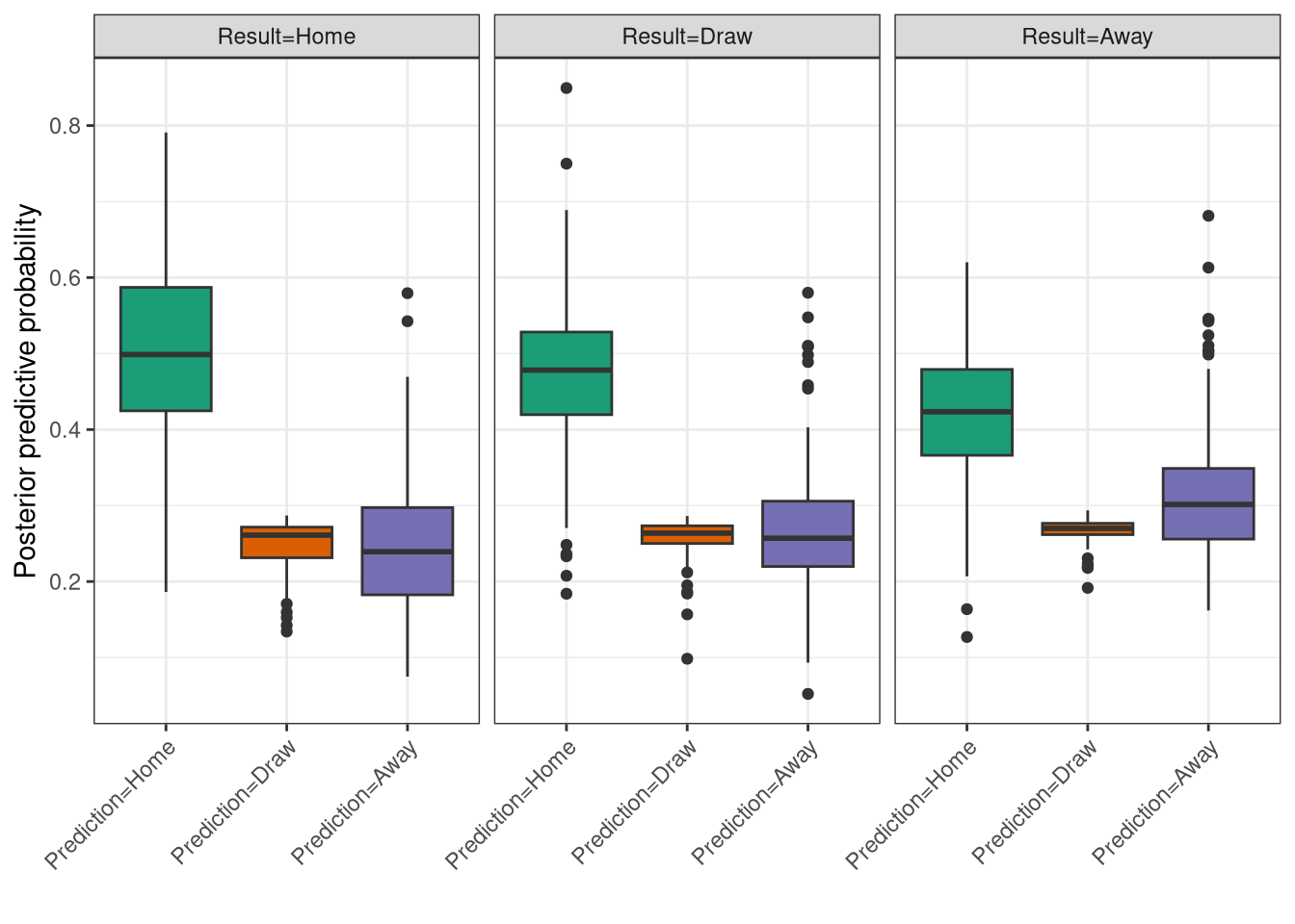
Prediction model - Poisson
In the 2018-2019 season the ordinal logistic regression match prediction model was replaced by a Poisson one in order to gain a more granular prediction rather than just Win/Loss/Draw, as well as opening up access to more betting markets. The likelihood is basically the same as before but now the skill difference is data (coming in from the Elo rating system) rather than parameters to be estimated. This allows for the use of a scaling $\beta$ coefficient, along with the usual league-specific intercepts $\alpha$.
$$\text{goals}_\text{home} \sim \text{Poisson}(\lambda_{\text{home},i})$$ $$\text{goals}_\text{away} \sim \text{Poisson}(\lambda_{\text{away},i})$$
$$\log(\lambda_{\text{home},i}) = \alpha_{\text{home},\text{leagues[i]}} + \beta_\text{home}(\psi_\text{home[i]} - \psi_\text{away[i]})$$ $$\log(\lambda_{\text{away},i}) = \alpha_{\text{away},\text{leagues[i]}} + \beta_\text{away}(\psi_\text{away[i]} - \psi_\text{home[i]})$$
The intercepts (number of goals scored with equal skill teams) $\alpha$ are shown in Figure 9 and are very similar to the values from the latent skill model last time, with the Bundesliga having more goals scored in general.
Show the code
mod_elo_poisson$coefs |>
    as_tibble() |>
    select(starts_with("alpha")) |>
    mutate(sample = row_number()) |>
    pivot_longer(
        -sample,
        names_pattern="alpha_(home|away)\\[([1-4])\\]",
        names_to=c("side", "league_id")
    ) |>
    mutate(
        league_id = as.integer(league_id),
        league = factor(league_id, levels=1:4, labels=mod_elo_poisson$leagues),
        league = factor(league, levels=league_ord, labels=league_labels),
        value = exp(value),
        side = factor(side, levels=c("home", "away"), labels=c("Home", "Away"))
    ) |>
    ggplot(aes(x=value, fill=league)) +
        geom_density() +
        facet_wrap(~side, ncol=1) +
        theme_minimal() +
        scale_fill_brewer("", palette="Dark2") +
        scale_x_continuous() +
        labs(x=latex2exp::TeX("Number of goals (derived from \\exp(\\alpha))")) +
        theme(
            legend.position = "bottom"
        )
Figure 9: Posterior $\alpha$ distribution from the Poisson match prediction model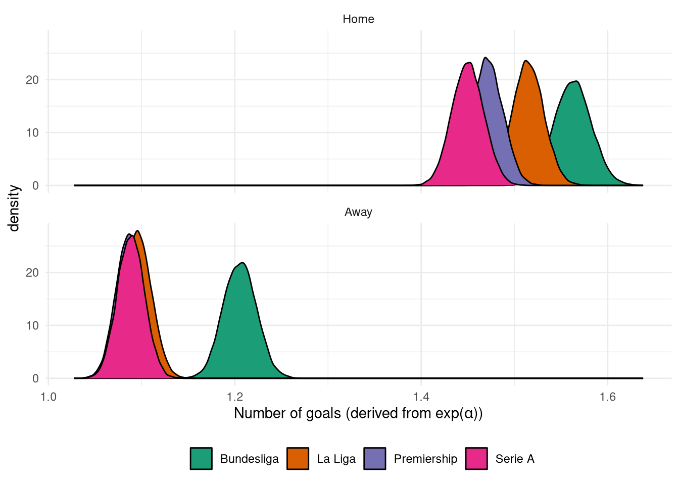
Meanwhile the $\beta$ coefficients are plotted in Figure 10. These are interpreteted as the multiplicative increase in the predicted number of goals scored for a 1-standard deviation increase in the skill difference. This is slightly cumbersome, mostly due to the “standard deviation increase in skill difference” bit, but this is necessary owing to the use of standardizing data inputs to improve MCMC efficiency by reducing the solution space. Anyway, the take-home message is that the skill difference has more of an impact on the home goals scored than away.
Show the code
mod_elo_poisson$coefs |>
    as_tibble() |>
    select(starts_with("beta")) |>
    mutate(
        sample = row_number(),
        beta_away = -beta_away  # Transform to be on same scale as home
    ) |>
    pivot_longer(
        -sample,
        names_pattern="beta_(home|away)",
        names_to=c("side")
    ) |>
    mutate(
        value = exp(value),
        side = factor(side, levels=c("home", "away"), labels=c("Home goals", "Away goals"))
    ) |>
    ggplot(aes(fill=side, x=value)) +
        geom_density(alpha=0.5) +
        theme_minimal() +
        scale_x_continuous() +
        scale_fill_manual("", values=c("lightblue", "lightsalmon")) +
        labs(x=latex2exp::TeX("$\\beta$")) +
        theme(
            legend.position = "bottom"
        )
Figure 10: Posterior $\beta$ distribution from the Poisson match prediction model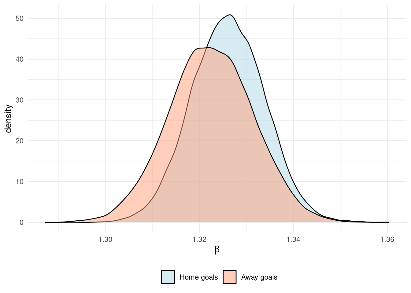
Figure 11 shows the posterior predictive distributions in terms of both goals scored and outcome probabilities for the Elo rating system applied to the 2005-2006 season only. The expected number of goals $\lambda$ increases/decreases exponentially with the skill difference, while the outcome probabilities look very similar to those from the ordinal model.
Show the code
predict_elo_poisson <- function(elo_diff, league) {
    coefs <- mod_elo_poisson$coefs

    league_num <- which(mod_elo_poisson$leagues == league)
    alpha_home_col <- paste0("alpha_home[", league_num, "]")
    alpha_away_col <- paste0("alpha_away[", league_num, "]")

    # Calculate lps
    elo_scale <- (elo_diff - mod_elo_poisson$elodiff_center) / mod_elo_poisson$elodiff_scale
    lambda_home <- exp(coefs[, alpha_home_col] + coefs[, "beta_home"] * elo_scale)
    lambda_away <- exp(coefs[, alpha_away_col] + coefs[, "beta_away"] * elo_scale)

    # Calculate predicted goals
    goals_home <- rpois(length(lambda_home), lambda_home)
    goals_away <- rpois(length(lambda_away), lambda_away)

    goal_prop_home <- table(goals_home) / length(goals_home)
    goal_prop_home <- tibble(
        name = sprintf("prop_goals_home_%s", names(goal_prop_home)),
        value=as.numeric(goal_prop_home)
    ) |> pivot_wider()
    goal_prop_away <- table(goals_away) / length(goals_away)
    goal_prop_away <- tibble(
        name = sprintf("prop_goals_away_%s", names(goal_prop_away)),
        value=as.numeric(goal_prop_away)
    ) |> pivot_wider()

    tibble(
        away_prob=mean(goals_away > goals_home),
        draw_prob=mean(goals_away == goals_home),
        home_prob=mean(goals_away < goals_home),
        goals_away_median = median(goals_away),
        goals_home_median = median(goals_home),
        goals_away_lower =quantile(goals_away, 0.025),
        goals_away_upper =quantile(goals_away, 0.975),
        goals_home_lower =quantile(goals_home, 0.025),
        goals_home_upper =quantile(goals_home, 0.975),
        lambda_home_median = median(lambda_home),
        lambda_home_lower =quantile(lambda_home, 0.025),
        lambda_home_upper =quantile(lambda_home, 0.975),
        lambda_away_median = median(lambda_away),
        lambda_away_lower =quantile(lambda_away, 0.025),
        lambda_away_upper =quantile(lambda_away, 0.975)
    ) |>
        cbind(goal_prop_home) |>
        cbind(goal_prop_away)
}
Show the code
pois_preds <- map_dfr(elo_diffs, predict_elo_poisson, "premiership", .id="elo_diff") |>
    mutate(
        elo_diff = as.integer(as.character(factor(as.integer(elo_diff), labels=elo_diffs)))
    )
p1 <- pois_preds |>
    select(elo_diff, starts_with("lambda")) |>
    pivot_longer(
        -elo_diff,
        names_pattern="lambda_(home|away)_(.+)",
        names_to=c("side", "statistic")
    ) |>
    pivot_wider(names_from=statistic, values_from = value) |>
    mutate(
        side = factor(side, levels=c("home", "away"), labels=c("Home", "Away"))
    ) |>
    ggplot(aes(x=elo_diff, colour=side, fill=side)) +
        geom_ribbon(aes(ymin=lower, ymax=upper), alpha=0.3) +
        geom_line(aes(y=median)) +
        theme_minimal() +
        labs(
            x=TeX("$\\psi_{home} - \\psi_{away}$"),
            y=TeX("Goal rate ($\\lambda$)")
        ) +
        theme(
            legend.position="bottom"
        ) +
        scale_colour_manual("", values=c("lightblue", "lightsalmon")) +
        scale_fill_manual("", values=c("lightblue", "lightsalmon"))

p2 <- pois_preds |>
    select(elo_diff, ends_with("prob")) |>
    pivot_longer(
        -elo_diff,
        names_pattern="(home|away|draw)_prob",
        names_to="side"
    ) |>
    mutate(
        side = factor(
            side,
            levels=c("home", "draw", "away"),
            labels=c("Home win", "Draw", "Away win")
        ),
        value = value * 100
    ) |>
    ggplot(aes(x=elo_diff, y=value, colour=side)) +
        geom_line() +
        theme_minimal() +
        scale_colour_manual("", values=c("lightblue", "forestgreen", "lightsalmon")) +
        geom_vline(xintercept=0, linetype="dashed", colour="orange") +
        annotate("label", x=0, y=80, label="Equal teams", colour="orange") +
        ylim(0, 100) +
        labs(x=TeX("$\\psi_{home} - \\psi_{away}$"), y="Probability of event (%)") +
        theme(
            legend.position="bottom"
        )

p1 + p2
Figure 11: Goal and match predictions from the Poisson model as a function of the rating difference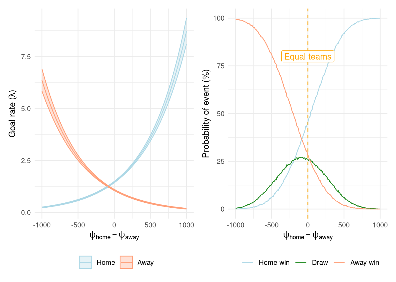
Finally, a posterior predictive check of the number of goals scored in the test season of 2005-2006 vs the modelled number is shown in Figure 12. The predictions aren’t as well calibrated as for the latent skill model, particularly for the away goals where too many away goals are forecasted. Although it’s worth again highlighting that this is over a single season without any time for the rating system to stabilize.
Show the code
pois_preds_ppc <- map_dfr(1:nrow(df_2005), function(i) {
    predict_elo_poisson(
        df_2005$home_elo[i] - df_2005$away_elo[i],
        df_2005$league[i]
    ) |>
        mutate(
            result = df_2005$result[i],
            date = df_2005$date[i],
            home = df_2005$home[i],
            away = df_2005$away[i]
        )
})
prop_actual <- df_2005 |>
    select(date, home, away, home_score, away_score) |>
    pivot_longer(c(home_score, away_score), names_to="side", values_to="goals") |>
    count(side, goals) |>
    group_by(side) |>
    mutate(
        pct = n / sum(n) * 100,
        side = gsub("_score", "", side),
        side = factor(side, levels=c("home", "away"),
                      labels =c("Home", "Away")),
        goals = factor(goals, levels=seq(0, 14))
    ) |>
    ungroup()

pois_preds_ppc |>
    select(date, home, away, starts_with("prop_goals")) |>
    pivot_longer(
        starts_with("prop_goals"),
        names_pattern = "prop_goals_(home|away)_([0-9]+)",
        names_to=c("side", "goals")
    ) |>
    mutate(
        goals = as.numeric(ifelse(is.na(goals), 0, goals)),
        side = factor(side, levels=c("home", "away"),
                      labels =c("Home", "Away")),
        pct = value * 100
    ) |>
    ggplot() +
        geom_boxplot(aes(x=as.factor(goals), y=pct)) +
        geom_col(aes(x=goals, y=pct), fill="orange", alpha=0.5, data=prop_actual) +
        facet_wrap(~side, nrow=1) +
        theme_bw() +
        labs(x="Number of goals", y="Percent")
Figure 12: Posterior predictive check of the Poisson model on the 2005-2006 Premiership season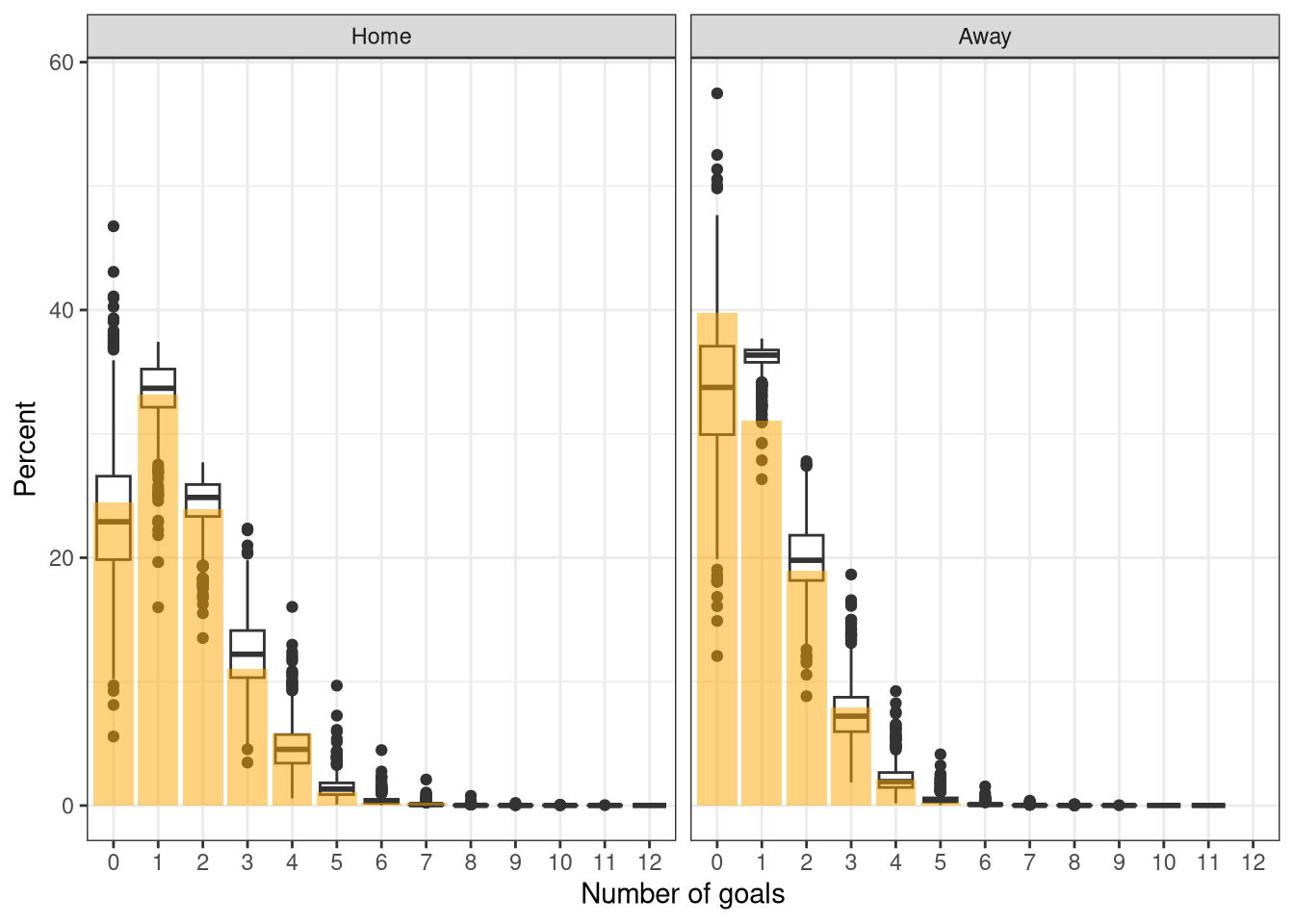
Next time we’ll look at consolidating this combination of Elo + separate model into a single parameterised system.