Introduction
This is the first in a retrospective series of posts looking at the evolution of Predictaball - my football match prediction engine - and reflect on how it mirrors my own development as a data scientist. I’ve been fortunate to work in a wide variety of domains, exposing me to a range of statistical paradigms and perspectives, which have been reflected in the models used in Predictaball. At the end of the series I’ll do a full comparison of all the algorithms too, as this is something I’ve never done before but have been interested in for a long time.
This first post will be focused on Bayesian statistics, and in particular hierarchical regression models, which were the models behind Predictaball for the 2016-2017 season.
Setup
First of all I’ll load all the packages I need, these are relatively standard packages for data wrangling and plotting/table generating, with the addition of cmdstanr for Stan (I prefer it to rstan as it uses the latest Stan) and e1071 for Naive Bayes classifiers.
NB: when I first fitted these types of models I was following Gelman & Hill as my reference, although I used JAGS rather than WinBUGS.
Show the code
library(tidyverse)
library(data.table)
library(e1071)        # Naive Bayes
library(cmdstanr)     # Bayesian regression
library(loo)          # pSIS calculation
library(knitr)        # Displaying tables
library(kableExtra)   # Displaying tables
library(ggrepel)      # Plotting
library(ggridges)     # Plotting
library(bayesplot)    # Plotting
options(knitr.table.html.attr = "quarto-disable-processing=true")
I already have a dataset comprising every football match from the top 4 European leagues (Premiership, La Liga, Serie A and Bundesliga, sorry France) going back to 2005-2006. In addition to the columns shown below, I also have created 4 columns assessing the form of the two teams by the number of wins and losses in their last 5 matches.
The first 10 seasons will be used as training data while the latter 10 will be used as a held-out test set for model comparison, although this will only be performed once at the very end once all models have been selected. This is a total of 14,460 matches for training - a decent number!
Show the code
df |>
    select(-ends_with("_win"), -ends_with("_draw"), -ends_with("_loss")) |>
    head() |>
    kable("html", col.names = c("League", "Season", "Date", "Home", "Away", "Home Score", "Away Score", "Result", "Dataset")) |>
    kable_styling(c("striped", "hover"), full_width=FALSE)
| League | Season | Date | Home | Away | Home Score | Away Score | Result | Dataset |
|---|---|---|---|---|---|---|---|---|
| laliga | 2024-2025 | 2025-05-25 | Athletic Bilbao | Barcelona | 0 | 3 | away | test |
| laliga | 2024-2025 | 2025-05-25 | Girona | Atletico Madrid | 0 | 4 | away | test |
| laliga | 2024-2025 | 2025-05-25 | Villarreal | Sevilla | 4 | 2 | home | test |
| premiership | 2024-2025 | 2025-05-25 | Bournemouth | Leicester | 2 | 0 | home | test |
| premiership | 2024-2025 | 2025-05-25 | Fulham | Man City | 0 | 2 | away | test |
| premiership | 2024-2025 | 2025-05-25 | Ipswich Town | West Ham | 1 | 3 | away | test |
Show the code
df |>
    count(dset) |>
    kable("html", col.names = c("Dataset", "Number of matches")) |>
    kable_styling(c("striped", "hover"), full_width=FALSE)
| Dataset | Number of matches |
|---|---|
| test | 14460 |
| training | 14460 |
Naive Bayes
The first model reflects how my first attempt at modelling football went, treating it as a standard classification problem based on a static feature vector. Here the features are simple, just the numbers of wins and losses per team in the last 5 matches of that season (the number of draws isn’t needed as this is collinear with the other features as it’s simply 5 - (n_wins + n_losses)). This should hopefully pick up a team’s current form, although it doesn’t account for longer term trends or the strength of their opponents in those last 5 matches. Because this is a very small feature space with only 4 features, each restricted to 6 values, a naive bayes classifier is a sensible option as anything more complex is likely to overfit.
It’s simple enough to fit the model using a familiar formula interface from the implementation in the e1071 package.
Show the code
mod_nb <- naiveBayes(
    result ~ home_win + home_loss + away_win + away_loss,
    data = df |>
         filter(dset == 'training') |>
         # Ensure both teams have played 5 games this season
         mutate(
             n_home = home_win + home_draw + home_loss,
             n_away = away_win + away_draw + away_loss
         ) |>
         filter(n_home == 5, n_away == 5)
)
The object shows both the marginal distribution of the result and the distributions of the predictor variables conditional on the result. The conditional probabilities are displayed with 1 table of 2 columns for each predictor, summarising the mean and standard deviation respectively.
For example, the second conditional probability table shows that matches that resulted in an away win had a home team with an average of 2.11 losses in the 5 leading games, compared to 1.74 in matches where the home team won. While being slightly awkward to think about, this makes sense - home teams that lost more historically are more likely to lose the current match.
Show the code
mod_nb
Naive Bayes Classifier for Discrete Predictors

Call:
naiveBayes.default(x = X, y = Y, laplace = laplace)

A-priori probabilities:
Y
     away      draw      home
0.2786492 0.2519206 0.4694302

Conditional probabilities:
      home_win
Y          [,1]     [,2]
  away 1.560310 1.108821
  draw 1.691868 1.142961
  home 2.020798 1.267030

      home_loss
Y          [,1]     [,2]
  away 2.116025 1.148188
  draw 1.996506 1.170955
  home 1.741902 1.172812

      away_win
Y          [,1]     [,2]
  away 2.202183 1.300969
  draw 1.914867 1.196221
  home 1.736447 1.153411

      away_loss
Y          [,1]     [,2]
  away 1.579552 1.154592
  draw 1.798920 1.143601
  home 1.949199 1.145573
This model has a training set accuracy of 48.5%, compared to a naive baseline of only predicting home wins (the modal class), which scores 46.9%. Without much additional context it’s hard to say whether 48.5% is a good accuracy for a challenging noisy problem, or it’s poor as it’s only slightly better than a naive benchmark.
Show the code
# Predicting on test data
y_pred <- predict(
    mod_nb,
    newdata = df |>
         filter(dset == 'training') |>
         mutate(
             n_home = home_win + home_draw + home_loss,
             n_away = away_win + away_draw + away_loss
             ) |>
         filter(n_home == 5, n_away == 5),
    )

df |>
 filter(dset == 'training') |>
 mutate(
     n_home = home_win + home_draw + home_loss,
     n_away = away_win + away_draw + away_loss
     ) |>
 filter(n_home == 5, n_away == 5) |>
 select(result) |>
 summarize(
     accuracy_nb = mean(result == y_pred)*100,
     accuracy_home_only = mean( result == 'home') * 100
 )
# A tibble: 1 × 2
  accuracy_nb accuracy_home_only
        <dbl>              <dbl>
1        48.5               46.9
It could be assumed that each league has slightly different probabilities (i.e. in a league with more stadium & climate variance we might expect to see fewer away wins) so instead it would make more sense to fit a separate model per league. However, this doesn’t result in a large increase in accuracy (48.7%), in which case it’s preferable to stick with the simpler model as hopefully this will generalize better.
Show the code
leagues <- levels(factor(df$league))
leagues <- setNames(leagues, leagues)
league_labels <- c("Bundesliga", "La Liga", "Premiership", "Serie A")
Show the code
mod_nb_leagues <- lapply(leagues, function(in_league) {
    naiveBayes(
        result ~ home_win + home_draw + home_loss + away_win + away_draw + away_loss,
        data = df |>
             filter(dset == 'training', league == in_league) |>
             mutate(
                 n_home = home_win + home_draw + home_loss,
                 n_away = away_win + away_draw + away_loss
                 ) |>
             filter(n_home == 5, n_away == 5)
    )
    }
)

# Predicting on test data
y_preds_league <- lapply(leagues, function(in_league) {
    preds <- predict(
        mod_nb_leagues[[in_league]],
        newdata = df |>
             filter(dset == 'training', league == in_league) |>
             mutate(
                 n_home = home_win + home_draw + home_loss,
                 n_away = away_win + away_draw + away_loss
                 ) |>
             filter(n_home == 5, n_away == 5),
    )
    actual <- df |>
             filter(dset == 'training', league == in_league) |>
             mutate(
                 n_home = home_win + home_draw + home_loss,
                 n_away = away_win + away_draw + away_loss
                 ) |>
             filter(n_home == 5, n_away == 5) |>
             pull(result)
    c(length(actual), sum(preds == actual))
})
sum(sapply(y_preds_league, function(x) x[2])) / sum(sapply(y_preds_league, function(x) x[1])) * 100
[1] 48.65557
Finally this model will be saved for later use when it is evaluated on the test seasons.
Show the code
saveRDS(mod_nb, "models/naive_bayes.rds")
Ordinal logistic model
The naive bayes model only has access to a very limited pool of information to make its prediction from. We can either try to increase the breadth of its knowledge base by adding more feature, some of which might be uninformative, or its depth by adding a small number of high quality features. Around this time I was starting to work with Bayesian hierarchical (aka multilevel) regression models in epidemiology, which inspired me to apply this to football match prediction to quantify each team’s latent skill through random effects.
This exposure to more rigorous statistical methods than just “throw everything into caret” also lead to the use of an ordinal categorical outcome, rather than just the regular categorical used in the naive bayes classifier, and indeed in much of the machine learning literature.
What this means in practice is that rather than “home win”, “away win”, “draw” being treated as 3 independent outcomes, instead this model uses their natural ordering (away win -> draw -> home win) to more accurately represent the structure. This is achieved in effect by having a linear predictor ($\phi$) which is used as the probability parameter in 2 different categorical draws, alongside 2 “cutpoints” ($k$) that provide the intercepts (the probability of each outcome when $\phi=0$). This can be summarised as follows:
$$\text{result}_i \sim \text{Ordered-logit}(\phi_i,k_i)$$
Here the linear predictor is simply the difference between the two teams’ latent skill levels ($\psi$).
$$\phi_i = \psi_\text{home[i]} - \psi_\text{away[i]}$$
While the intercept is specific to each league (this wasn’t found to make much difference for the Naive Bayes model but incorporating known hierarchical relationships in multi-level models can make more efficient use of the data).
$$k_i = \kappa_{\text{league[i]}}$$ Both the skill and cutpoint parameters have uninformative hyper-priors, since both of these are hierarchical (there are 135 teams and 4 leagues).
$$\psi \sim \text{Normal}(\mu_\psi, \sigma_\psi)$$
$$\kappa \sim \text{Normal}(\mu_\kappa, \sigma_\kappa)$$
$$\mu_\psi \sim \text{Normal}(0, 1)$$ $$\sigma_\psi \sim \text{Half-Normal}(0, 2.5)$$
$$\mu_\kappa \sim \text{Normal}(0, 1)$$ $$\sigma_\kappa \sim \text{Half-Normal}(0, 2.5)$$
Here’s the model in Stan code.
data {
  int<lower=3> N_outcomes;
  int<lower=0> N_matches;
  int<lower=0> N_teams;
  int<lower=0> N_leagues;
  array[N_matches] int<lower=1, upper=N_outcomes> result;
  array[N_matches] int<lower=1, upper=N_teams> home;
  array[N_matches] int<lower=1, upper=N_teams> away;
  array[N_matches] int<lower=1, upper=N_leagues> league;
}
parameters {
  real skill_mu;
  real<lower=0> skill_sigma;
  array[N_leagues] ordered[N_outcomes - 1] cutpoints;
  ordered[N_outcomes - 1] cutpoints_mu;
  vector<lower=0>[N_outcomes-1] cutpoints_sigma;
  vector[N_teams] skill_raw;
}
transformed parameters {
  vector[N_teams] skill;
  skill = skill_mu + skill_sigma * skill_raw;
}
model {

  skill_mu ~ normal(0, 1);
  skill_sigma ~ normal(0, 2.5);
  cutpoints_mu ~ normal(0, 1);
  cutpoints_sigma ~ normal(0, 2.5);
  for (j in 1:N_leagues) {
      cutpoints[j] ~ normal(cutpoints_mu, cutpoints_sigma);
  }
  skill_raw ~ std_normal();
  for (n in 1:N_matches) {
    result[n] ~ ordered_logistic((skill[home[n]] - skill[away[n]]), cutpoints[league[n]]);
  }
}
Now for some data preparation. Firstly obtain the set of teams that are present in the training data as only these will have their latent skill directly estimated. Any new teams in the test set (i.e. through promotion) will use the random effects to draw a random skill level from the distribution over teams.
Show the code
training_teams <- df |>
    filter(dset == 'training') |>
    distinct(home) |>
    pull(home)
And prepare inputs for sampling.
Show the code
fit_ord_log_2 <- mod_ord_log_2$sample(
    data = list(
        N_outcomes = 3,
        N_matches = sum(df$dset == 'training'),
        N_teams = length(training_teams),
        N_leagues=length(unique(df$league)),
        result = df |>
            filter(dset == 'training') |>
            mutate(result_fact = as.integer(factor(result, levels=c("away", "draw", "home")))) |>
            pull(result_fact),
        home = df |>
            filter(dset == 'training') |>
            mutate(home_fact = as.integer(factor(home, levels=training_teams))) |>
            pull(home_fact),
        away = df |>
            filter(dset == 'training') |>
            mutate(away_fact = as.integer(factor(away, levels=training_teams))) |>
            pull(away_fact),
        league = df |>
            filter(dset == 'training') |>
            mutate(league_fact = as.integer(factor(league, levels=leagues))) |>
            pull(league_fact)
    ),
    parallel_chains = 4
)
fit_ord_log_2$save_object("models/hierarchical_ordinal_league.rds")
Having 7% transitions is a bit worrying and potentially indicative of an awkward sampling geometry so it’s worth digging into, although we can take reassurance that all Rhats are <= 1.01.
Show the code
fit_ord_log_2$diagnostic_summary()
Warning: 277 of 4000 (7.0%) transitions ended with a divergence.
See https://mc-stan.org/misc/warnings for details.

$num_divergent
[1] 56 92 49 80

$num_max_treedepth
[1] 0 0 0 0

$ebfmi
[1] 0.6519939 0.7062917 0.8185837 0.7758938
There is very little variance in the sampling of $\sigma_\psi$ and $\kappa$ (Figure 1) potentially there is a more efficient way of encoding an ordered logistic regression in Stan, or perhaps the priors need a bit of tweaking. The divergences occur when the samples for these parameters are close to the mean.
Show the code
color_scheme_set("darkgray")
# for the second model
all_vars <- c("skill_mu", "skill_sigma", "skill", "cutpoints_mu", "cutpoints_sigma", "cutpoints")
lp_ord <- log_posterior(fit_ord_log_2)
np_ord <- nuts_params(fit_ord_log_2)

mcmc_parcoord(fit_ord_log_2$draws(variables=c("skill_mu", "skill_sigma", sprintf("skill[%d]", 1:10), "cutpoints_mu", "cutpoints_sigma", "cutpoints")), np = np_ord) +
    theme(
        axis.text.x = element_text(angle=90)
    )
Figure 1: Parallel coordinate plot of MCMC sampling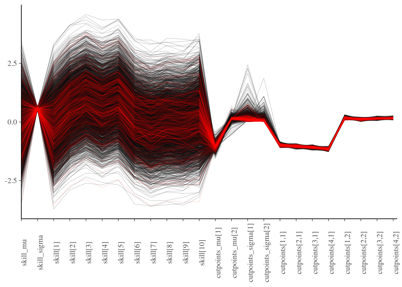
This poor exploration is also visible in the trace plots in Figure 2.
Show the code
color_scheme_set("mix-brightblue-gray")
mcmc_trace(fit_ord_log_2$draws(variables = c("skill_mu", "skill_sigma", "cutpoints", "cutpoints_mu", "cutpoints_sigma"), format="draws_matrix", inc_warmup=F))
Figure 2: Diagnostic MCMC trace plots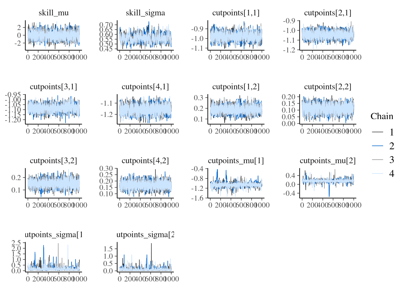
These divergences don’t affect the model’s log probability (top plot in Figure 3), and only a fraction impact the acceptance (bottom plot), so we’ll just move forward for now.
Show the code
color_scheme_set("red")
mcmc_nuts_divergence(np_ord, lp_ord)
Figure 3: Divergences vs log-probability and acceptance rate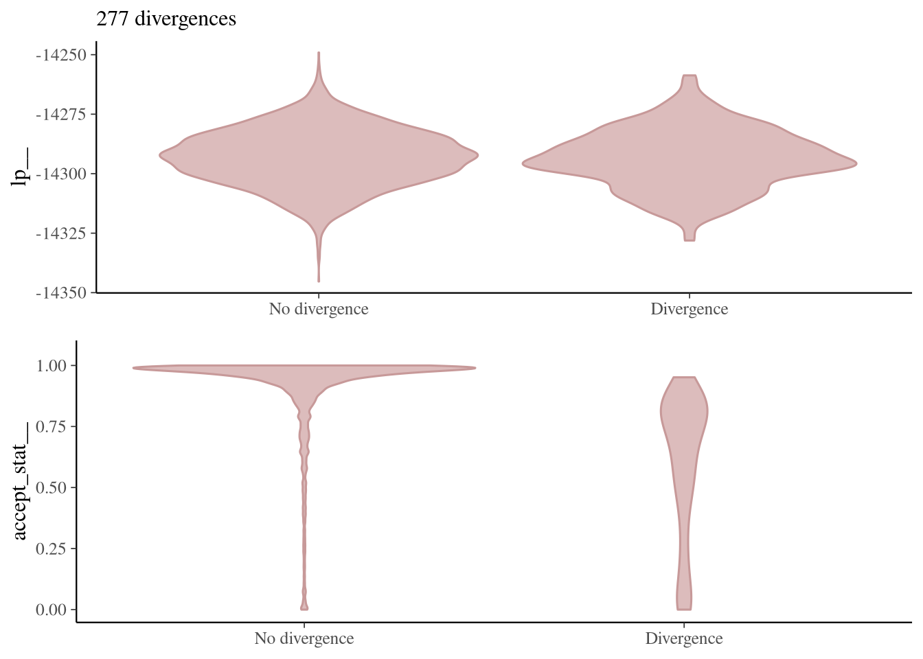
And finally to looking at the parameters themselves! Figure 4 shows the posterior distributions of $\kappa$ for each league, which have been back-transformed into the 3 outcome possibilities. It’s interesting to note that while all 4 leagues have very similar home win probabilities, there is much more spread in the other two outcomes, with the Bundesliga in particular having the highest away win probability. Serie A on the other hand looks to have the strongest home stadium effect, as it has the lowest away win probability.
Show the code
inv_logit <- function(x) {
    exp(x) / (1 + exp(x))
}

cutpoints_df <- fit_ord_log_2$draws(variables="cutpoints", format="draws_matrix")  |>
    as_tibble() %>%
    mutate(sample=1:nrow(.)) |>
    pivot_longer(-sample) |>
    mutate(
        league_id = as.integer(str_extract(name, "\\[([1-4])", group=1)),
        cutpoint_id = as.integer(str_extract(name, ",([1-4])\\]", group=1)),
        league = levels(factor(df$league))[league_id]
    ) |>
    select(sample, league, cutpoint_id, value) |>
    mutate(
        value_trans = inv_logit(value),
    )
cutpoints_df |>
    select(sample, league, cutpoint_id, value_trans) |>
    pivot_wider(names_from = "cutpoint_id", values_from="value_trans") |>
    mutate(
        `3` = 1 - `2`,
        `2` = `2` - `1`
    ) |>
    pivot_longer(c(`1`, `2`, `3`)) |>
    mutate(
        event = factor(name, levels=c(3, 2, 1), labels=c("Home win", "Draw", "Away win")),
        league = factor(league, levels=leagues, labels=league_labels)
    ) |>
    ggplot(aes(x=value, group=league, fill=league)) +
        geom_density() +
        facet_wrap(~event, ncol=1) +
        theme_minimal() +
        scale_fill_brewer("", palette="Dark2") +
        scale_x_continuous() +
        labs(x=latex2exp::TeX("Probability of event (inv_logit(\\kappa))")) +
        theme(
            legend.position = "bottom"
        )
Figure 4: Plot of outcome probabilities derived from $\kappa$ from ordinal logistic regression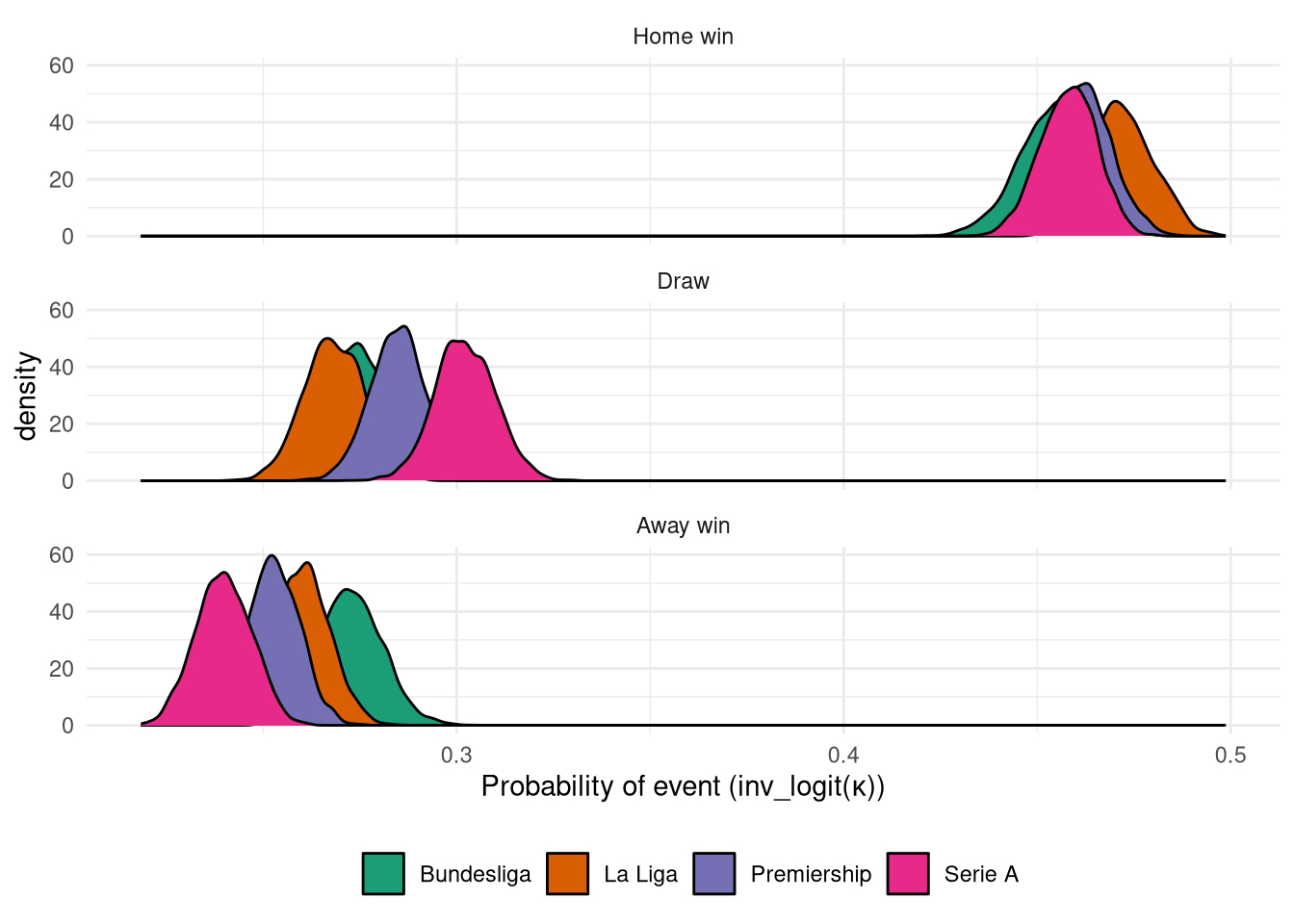
The other main parameter is the latent skill factors $\psi$, which are summarised in Figure 5 alongside the team standing at the end of the final training season. NB: the median $\psi$ for each team is shown to reduce clutter. Overall the skill levels that are calculated over the previous ten seasons line up quite highly with the final league positions at the end of those ten years, indicating that on the whole, a team’s skill level is relatively constant from season to season. There are some exceptions, like Milan who came in 10th in 2014-2015 but had the 3rd best performance over the full 2004-2015 period. I would expect that a sport like American football or ice hockey, where there are policies in place to even the playing field, would have a weaker relationship.
Show the code
league_positions_training <- tribble(
    ~league, ~position, ~team,
    "premiership", 1, "Chelsea",
    "premiership", 2, "Man City",
    "premiership", 3, "Arsenal",
    "premiership", 4, "Man Utd",
    "premiership", 5, "Tottenham",
    "premiership", 6, "Liverpool",
    "premiership", 7, "Southampton",
    "premiership", 8, "Swansea",
    "premiership", 9, "Stoke",
    "premiership", 10, "Crystal Palace",
    "premiership", 11, "Everton",
    "premiership", 12, "West Ham",
    "premiership", 13, "West Brom",
    "premiership", 14, "Leicester",
    "premiership", 15, "Newcastle",
    "premiership", 16, "Sunderland",
    "premiership", 17, "Aston Villa",
    "premiership", 18, "Hull",
    "premiership", 19, "Burnley",
    "premiership", 20, "QPR",
    "laliga", 1, "Barcelona",
    "laliga", 2, "Real Madrid",
    "laliga", 3, "Atletico Madrid",
    "laliga", 4, "Valencia",
    "laliga", 5, "Sevilla",
    "laliga", 6, "Villarreal",
    "laliga", 7, "Athletic Bilbao",
    "laliga", 8, "Celta Vigo",
    "laliga", 9, "Malaga",
    "laliga", 10, "Espanyol",
    "laliga", 11, "Rayo Vallecano",
    "laliga", 12, "Real Sociedad",
    "laliga", 13, "Elche",
    "laliga", 14, "Levante",
    "laliga", 15, "Getafe",
    "laliga", 16, "La Coruna",
    "laliga", 17, "Granada",
    "laliga", 18, "Eibar",
    "laliga", 19, "Almeria",
    "laliga", 20, "Cordoba",
    "seriea", 1, "Juventus",
    "seriea", 2, "Roma",
    "seriea", 3, "Lazio",
    "seriea", 4, "Fiorentina",
    "seriea", 5, "Napoli",
    "seriea", 6, "Genoa",
    "seriea", 7, "Sampdoria",
    "seriea", 8, "Inter",
    "seriea", 9, "Torino",
    "seriea", 10, "Milan",
    "seriea", 11, "Palermo",
    "seriea", 12, "Sassuolo",
    "seriea", 13, "Verona",
    "seriea", 14, "Chievo",
    "seriea", 15, "Empoli",
    "seriea", 16, "Udinese",
    "seriea", 17, "Atalanta",
    "seriea", 18, "Cagliari",
    "seriea", 19, "Cesena",
    "seriea", 20, "Parma",
    "bundesliga1", 1, "Bayern Munich",
    "bundesliga1", 2, "Wolfsburg",
    "bundesliga1", 3, "Borussia Moenchengladbach",
    "bundesliga1", 4, "Bayern Leverkusen",
    "bundesliga1", 5, "Augsburg",
    "bundesliga1", 6, "Schalke",
    "bundesliga1", 7, "Borussia Dortmund",
    "bundesliga1", 8, "Hoffenheim",
    "bundesliga1", 9, "Ein Frankfurt",
    "bundesliga1", 10, "Werder Bremen",
    "bundesliga1", 11, "Mainz",
    "bundesliga1", 12, "Koln",
    "bundesliga1", 13, "Hannover",
    "bundesliga1", 14, "Stuttgart",
    "bundesliga1", 15, "Hertha",
    "bundesliga1", 16, "Hamburg",
    "bundesliga1", 17, "Freiburg",
    "bundesliga1", 18, "Paderborn"
)
skills_ordinal <- fit_ord_log_2$draws(variables="skill", format="draws_df") |>
    as_tibble() |>
    mutate(
        sample=row_number()
    ) |>
    pivot_longer(-sample) |>
    mutate(
        teamid = as.integer(str_extract(name, "skill\\[([0-9]+)\\]", group = 1)),
        team = training_teams[teamid]
    ) |>
    group_by(team) |>
    summarise(
        median = median(value),
        lower=quantile(value, 0.025),
        upper = quantile(value, 0.975)
    ) |>
    ungroup() |>
    inner_join(league_positions_training, by="team") |>
    mutate(league_label = factor(league, levels=leagues, labels=league_labels))

skills_ordinal |>
    ggplot(aes(x=median, y=position)) +
        geom_point(shape=21, size=2) +
        scale_y_reverse() +
        geom_smooth(method="lm") +
        geom_label_repel(
            aes(label=team),
            data=skills_ordinal |>
                filter(team %in% c(
                    "Bayern Munich",
                    "Barcelona",
                    "Real Madrid",
                    "Chelsea",
                    "Juventus",
                    "Milan",
                    "Inter",
                    "Borussia Moenchengladbach",
                    "Augsburg",
                    "Wolfsburg",
                    "Aston Villa",
                    "Parma",
                    "Genoa",
                    "Lazio",
                    "Sampdoria",
                    "QPR",
                    "Paderborn",
                    "Cordoba",
                    "Cesena"
                ))
        ) +
        labs(x=latex2exp::TeX("Median \\psi"), y="League position") +
        facet_wrap(~league_label, scales="free") +
        theme_bw()
Figure 5: Relationship between $\psi$ and a team’s final standing at the end of the training set.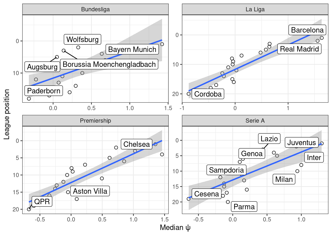
Next we want to run a posterior predictive check to see if the simulated outcomes using the full model posterior matches up with the actual match results. This is achieved by running each match through each of the 4,000 posterior draws, drawing a match result from the ordinal logistic regression, and calculating the probability of each outcome for that match as the number of outcomes / 4000.
Show the code
skills_post <- fit_ord_log_2$draws(c("skill"), format="draws_matrix") |> as.matrix()
cutpoints_post <- fit_ord_log_2$draws(c("cutpoints"), format="draws_matrix") |> as.matrix()
train_df <- df |>
    filter(dset == 'training') |>
    select(home, away, league) |>
    mutate(
        home_id = as.integer(factor(home, levels=training_teams)),
        away_id = as.integer(factor(away, levels=training_teams)),
        league_id = as.integer(factor(league, levels=leagues))
    ) |>
    select(home_id, away_id, league_id)

get_probabilities <- function(phi, kappa) {
    # phi is 1d array
    # kappa is 2d array
    N_samples <- length(phi)
    q <- inv_logit(kappa - phi)
    probs <- matrix(nrow=N_samples, ncol=3)
    probs[, 1] <- q[, 1]
    probs[, 2] <- q[, 2] - q[, 1]
    probs[, 3] <- 1 - q[, 2]
    probs
}

rordlogit_vectorized <- function(phi, kappa) {
    probs <- get_probabilities(phi, kappa)
    cumprobs <- t(apply(probs, 1, cumsum))
    thresh <- runif(nrow(probs))
    apply(cumprobs > thresh, 1, which.max)
}

outcomes <- matrix(nrow=4000, ncol=sum(df$dset == 'training'))
for (i in 1:nrow(train_df)) {
    cat(sprintf("%d/%d\n", i, nrow(train_df)))
    start <- (i-1)*4000 + 1
    end <- i*4000
    phi_i <- as.vector(skills_post[, train_df$home_id[i]] - skills_post[, train_df$away_id[i]])
    kappa_i <- as.matrix(cutpoints_post[, c(train_df$league_id[i], train_df$league_id[i]+4)])
    outcomes[, i] <- rordlogit_vectorized(phi_i, kappa_i)
}
Show the code
outcome_counts <- apply(outcomes, 2, table)
outcome_probs <- t(outcome_counts / colSums(outcome_counts))
Figure 6 shows the results, where each of the 3 panels refers to each of the 3 actual match outcomes, and the boxplots give the corresponding predictions. What we’d ideally see is that in the Home result panel, home results are predicted 100% of the time and draws and away wins have 0%. However of course this is unrealistic. Instead we see that home win is predicted the most often, even in away wins, highlighting the significant home advantage in football. It is reassuring to see that away win is narrowly the next most often predicted outcomes for away matches. Although strikingly draws are both the lowest predicted outcome in matches that did end in draws, and also have the lowest range of probabilities, suggesting that this is the outcome that is hardest to predict.
Show the code
df |>
    filter(dset == 'training') |>
    select(league, date, home_team=home, away_team=away, result) |>
    mutate(
        away= outcome_probs[, 1],
        draw= outcome_probs[, 2],
        home= outcome_probs[, 3]
    ) |>
    pivot_longer(c(away, draw, home)) |>
    mutate(
        result = factor(result, levels=c('home', 'draw', 'away'), labels=c('Result=Home', 'Result=Draw', 'Result=Away')),
        name = factor(name, levels=c('home', 'draw', 'away'), labels=c('Prediction=Home', 'Prediction=Draw', 'Prediction=Away'))
    ) |>
    ggplot(aes(x=name, y=value, fill=name)) +
        geom_boxplot() +
        facet_wrap(~result) +
        theme_bw() +
        scale_fill_brewer("Modelled outcome", palette="Dark2") +
        labs(x="", y="Posterior predictive probability") +
        guides(fill="none") +
        theme(
            legend.position = "bottom",
            axis.text.x = element_text(angle=45, hjust=1)
        )
Figure 6: Posterior predictive check of the ordinal logistic regression model.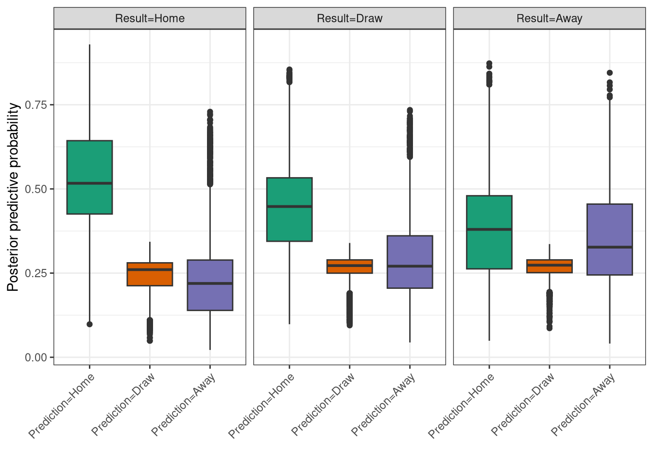
Poisson model
Football matches aren’t simply win/loss/draw like chess games are, those outcomes are derived from the number of goals scored by each team. The number of goals scored the therefore contain more information than simply the outcome, i.e. an 8-0 rout is very different to a scrappy 1-0 win. It’s possible therefore that using the number of goals scored by both teams will allow for more accurate skill estimates. Fortunately, using generalized linear models makes it easy to change from a results-based outcome to a goals-based one by swapping out the ordinal logistic likelihood for something that works with goals. Goals are discrete integers, so the default option is the Poisson distribution. This model then looks as follows, where we still use the difference between latent team skill factors ($\psi$), but the intercepts ($\alpha$) are now directly incorporated into the linear predictor rather than being separate distributional parameters. The priors and hyper-priors are the same as before.
$$\text{goals}_\text{home} \sim \text{Poisson}(\lambda_{\text{home},i})$$ $$\text{goals}_\text{away} \sim \text{Poisson}(\lambda_{\text{away},i})$$
$$\log(\lambda_{\text{home},i}) = \alpha_{\text{home},\text{leagues[i]}} + \psi_\text{home[i]} - \psi_\text{away[i]}$$ $$\log(\lambda_{\text{away},i}) = \alpha_{\text{away},\text{leagues[i]}} + \psi_\text{away[i]} - \psi_\text{home[i]}$$
The full Stan code is displayed below. This Poisson model was never actually used directly in the live Predictaball website, but a modified version of it was, as will be explained in the next post.
data {
  int<lower=0> N_matches;
  int<lower=0> N_teams;
  int<lower=0> N_leagues;
  array[N_matches] int goals_home;
  array[N_matches] int goals_away;
  array[N_matches] int<lower=1, upper=N_teams> home;
  array[N_matches] int<lower=1, upper=N_teams> away;
  array[N_matches] int<lower=1, upper=N_leagues> league;
}
parameters {
  real skill_mu;
  real<lower=0> skill_sigma;
  vector[N_teams] skill_raw;
  vector[N_leagues] alpha_home_raw;
  vector[N_leagues] alpha_away_raw;
  real alpha_home_mu;
  real<lower=0> alpha_home_sigma;
  real alpha_away_mu;
  real<lower=0> alpha_away_sigma;
}
transformed parameters {
  vector[N_leagues] alpha_home;
  vector[N_leagues] alpha_away;
  vector[N_teams] skill;
  alpha_home = alpha_home_mu + alpha_home_sigma * alpha_home_raw;
  alpha_away = alpha_away_mu + alpha_away_sigma * alpha_away_raw;
  skill = skill_mu + skill_sigma * skill_raw;
}
model {
  alpha_home_mu ~ normal(0, 1);
  alpha_home_sigma ~ normal(0, 2.5);
  alpha_away_mu ~ normal(0, 1);
  alpha_away_sigma ~ normal(0, 2.5);
  alpha_home_raw ~ std_normal();
  alpha_away_raw ~ std_normal();
  skill_mu ~ normal(0, 1);
  skill_sigma ~ normal(0, 2.5);
  skill_raw ~ std_normal();
  for (n in 1:N_matches) {
    goals_home[n] ~ poisson(exp(alpha_home[league[n]] + skill[home[n]] - skill[away[n]]));
    goals_away[n] ~ poisson(exp(alpha_away[league[n]] + skill[away[n]] - skill[home[n]]));
  }
}
Show the code
mod_pois_2 <- cmdstan_model("models/hierarchical_poisson_1score_league.stan")
Show the code
fit_pois_2 <- mod_pois_2$sample(
    data = list(
        N_matches = sum(df$dset == 'training'),
        N_teams = length(training_teams),
        N_leagues=length(unique(df$league)),
        goals_home = df |>
            filter(dset == 'training') |>
            pull(home_score) |>
            as.integer(),
        goals_away = df |>
            filter(dset == 'training') |>
            pull(away_score) |>
            as.integer(),
        home = df |>
            filter(dset == 'training') |>
            mutate(home_fact = as.integer(factor(home, levels=training_teams))) |>
            pull(home_fact),
        away = df |>
            filter(dset == 'training') |>
            mutate(away_fact = as.integer(factor(away, levels=training_teams))) |>
            pull(away_fact),
        league = df |>
            filter(dset == 'training') |>
            mutate(league_fact = as.integer(factor(league, levels=leagues))) |>
            pull(league_fact)
    ),
    parallel_chains = 4
)
fit_pois_2$save_object("models/hierarchical_poisson_1score_league.rds")
The number of divergences has now decreased to 1%, presumably because the Poisson likelihood is far more simple than the ordinal one, and Rhats are all < 1.02 so I’ll not display the diagnostic plots to save space and instead jump straight to the estimated parameters.
Show the code
fit_pois_2$diagnostic_summary()
Warning: 25 of 4000 (1.0%) transitions ended with a divergence.
See https://mc-stan.org/misc/warnings for details.

$num_divergent
[1] 18  3  2  2

$num_max_treedepth
[1] 0 0 0 0

$ebfmi
[1] 0.6361676 0.6661691 0.7298566 0.7047161
Show the code
color_scheme_set("darkgray")
# for the second model
all_vars <- c("skill_mu", "skill_sigma", sprintf("skill[%d]", 1:10), "alpha_home", "alpha_away", "alpha_home_mu", "alpha_away_mu", "alpha_home_sigma", "alpha_away_sigma")
lp_ord <- log_posterior(fit_pois_2)
np_ord <- nuts_params(fit_pois_2)

mcmc_parcoord(fit_pois_2$draws(variables=all_vars), np = np_ord) +
    theme(
        axis.text.x = element_text(angle=90)
    )
Show the code
# Main issue is in the group level intercept
color_scheme_set("mix-brightblue-gray")
#mcmc_trace(posterior_cp, pars = "tau", np = np_cp) +
#  xlab("Post-warmup iteration")
mcmc_trace(fit_pois_2$draws(variables = c("skill_mu", "skill_sigma", "alpha_home", "alpha_away", "alpha_home_mu", "alpha_away_mu", "alpha_home_sigma", "alpha_away_sigma"), format="draws_matrix", inc_warmup=F))
Show the code
# Likewise doesn't really affect log prob or acceptance
color_scheme_set("red")
mcmc_nuts_divergence(np_ord, lp_ord)
Figure 7 shows the posterior distribution of $\alpha$, i.e. the expected number of goals scored by each side when there is no skill difference. As expected home teams score more than away teams with 1.5 goals on average compared to 1.1 Interestingly the Bundesliga is an outlier with closer to 1.2 away goals on average, which supports the finding from the previous model that away wins are more common in this league. Although rather than being indicative of a more balanced league, the Bundesliga also features more home goals too, so perhaps it’s just a high scoring league in general.
Figure 7: Posterior of $\exp(\alpha)$ from Poisson model.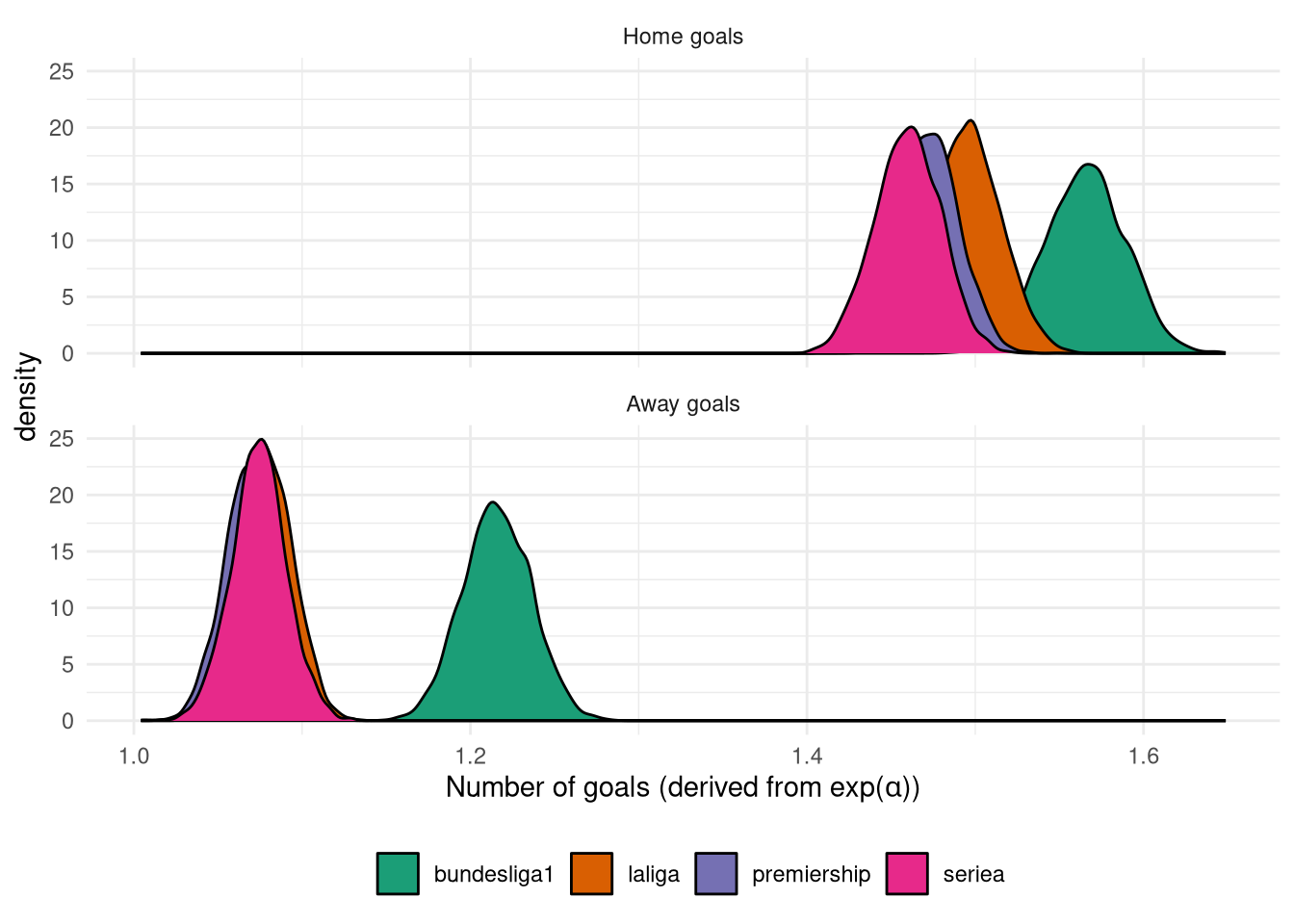
The distribution of team scores ($\psi$) are shown in Figure 8, alongside those from the Ordinal logistic regression model. It’s immediately apparent that there is far higher spread of team skill levels in the Ordinal logistic regression model compared to the Poisson, which is due to the fact that these values aren’t directly comparable, since 1 unit of $\psi$ in the Poisson model corresponds to an increase in the log count of goals of 1, whereas in the ordinal logistic regression it is an increase of 1 in the cumulative log-odds.
Figure 8: Comparison of $\psi$ between the Ordinal Logistic and Poisson models.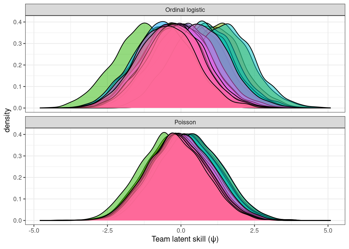
Instead it is fairer to compare the skill levels on their relative rankings, as in the table below. Here we can see that they are largely in agreement, especially for the top 8 teams. The team they disagree on the most is Leicester, who according to their match rankings are 25th, but by their goals scored they are 11th, a massive difference of 14 places!
| Team | Ordinal rank | Poisson rank | Difference between ranks |
|---|---|---|---|
| Man Utd | 1 | 1 | 0 |
| Chelsea | 2 | 2 | 0 |
| Arsenal | 3 | 3 | 0 |
| Liverpool | 4 | 4 | 0 |
| Man City | 5 | 5 | 0 |
| Tottenham | 6 | 6 | 0 |
| Everton | 7 | 7 | 0 |
| Southampton | 8 | 8 | 0 |
| Aston Villa | 9 | 10 | 1 |
| Swansea | 12 | 9 | 3 |
| Blackburn | 10 | 14 | 4 |
| Stoke | 11 | 13 | 2 |
| Leicester | 25 | 11 | 14 |
| Crystal Palace | 15 | 12 | 3 |
| Newcastle | 13 | 15 | 2 |
| West Ham | 16 | 16 | 0 |
| Fulham | 14 | 17 | 3 |
| Bolton | 18 | 18 | 0 |
| Portsmouth | 17 | 19 | 2 |
| Middlesbrough | 20 | 20 | 0 |
| West Brom | 22 | 21 | 1 |
| Reading | 27 | 22 | 5 |
| Birmingham | 21 | 23 | 2 |
| Sunderland | 29 | 24 | 5 |
| Charlton | 24 | 25 | 1 |
| Sheffield Utd | 28 | 26 | 2 |
| Norwich | 19 | 27 | 8 |
| Wigan | 23 | 28 | 5 |
| Blackpool | 26 | 29 | 3 |
| Hull | 30 | 30 | 0 |
| QPR | 35 | 31 | 4 |
| Watford | 32 | 32 | 0 |
| Wolves | 31 | 33 | 2 |
| Burnley | 34 | 34 | 0 |
| Cardiff | 33 | 35 | 2 |
| Derby | 36 | 36 | 0 |
As with the ordinal logistic regression, we want to check that the model’s outputs reflect the data. Fortunately this is a bit easier with the Poisson model as we can directly compare the number of goals scored to that predicted, as shown in Figure 9 where the orange bars show the actual proportion of games with each number of goals, and the boxplots show the proportion of each number of goals scored for each match. Unlike the ordinal logistic regression they match up very well with the posterior medians (thick line in middle of boxplots), although there are long tails on the predicted distributions, particularly for 0. It’s reassuring to see that the model allows for sufficient variance to model the full range of goals scored - as Poisson models are limited by having the variance = the mean count - so overdispersion often occurs. This is usually fixed by separately modelling the variance.
Show the code
prop_actual <- df |>
    filter(dset == 'training') |>
    select(date, home, away, home_score, away_score) |>
    pivot_longer(c(home_score, away_score), names_to="side", values_to="goals") |>
    count(side, goals) |>
    group_by(side) |>
    mutate(
        pct = n / sum(n) * 100,
        side = gsub("_score", "", side),
        side = factor(side, levels=c("home", "away"),
                      labels =c("Home", "Away")),
        goals = factor(goals, levels=seq(0, 14))
    ) |>
    ungroup()

pred_outcomes |>
    mutate(
        side = factor(side, levels=c("home", "away"),
                      labels =c("Home", "Away")),
        pct = prop * 100,
        goals = factor(goals, levels=seq(0, 14))
    ) |>
    ggplot() +
        geom_boxplot(aes(x=as.factor(goals), y=pct)) +
        geom_col(aes(x=goals, y=pct), fill="orange", alpha=0.5, data=prop_actual) +
        facet_wrap(~side, nrow=1) +
        theme_bw() +
        labs(x="Number of goals", y="Percent")
Figure 9: Posterior predictive check of Poisson model.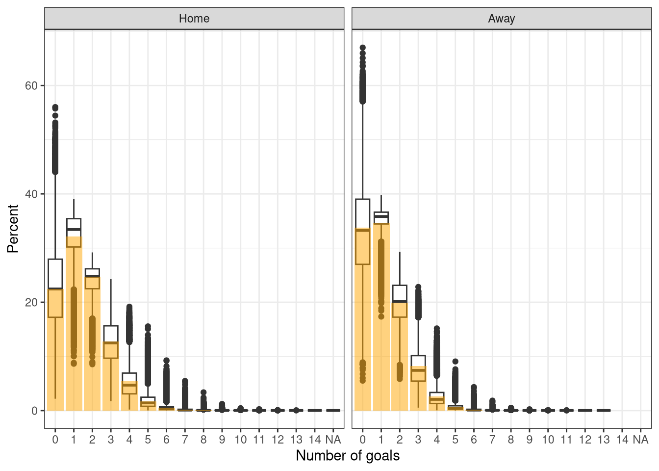
Poisson with attack & defend skills
All the models thus far have summarised a team’s ability to win matches or score goals into a single score, which makes modelling nice and convenient. However, this is a drastic simplification of a team’s strengths and weaknesses. A simple extension of the 1-skill level abstraction is to use 2 factors: one for attacking and one for defending. This can be done by modifying the linear predictor part of the likelihood as follows, so that the number of goals scored by a team is the difference between its attacking score and the opposition’s defence score.
$$\log(\lambda_{\text{home},i}) = \alpha_{\text{home},\text{leagues[i]}} + \psi^\text{attack}_\text{home[i]} - \psi^\text{defend}_\text{away[i]}$$ $$\log(\lambda_{\text{away},i}) = \alpha_{\text{away},\text{leagues[i]}} + \psi^\text{attack}_\text{away[i]} - \psi^\text{defend}_\text{home[i]}$$
Because both of these factors are likely to be correlated (a team that is good at scoring will likely also be good at defending owing to financial resources & being coached well), we can draw these two scores from an underlying score for each team, much like we had before. This $\psi$ aims to represent the overall ability of a team, so we would hopefully expect to see it correlate with $\psi$ from the single-score Poisson model.
$$\psi^\text{attack}_i, \psi^\text{defend}_i \sim \text{Normal}(\psi_i, 2.5)$$
NB: I tried to model this relationship using a multi-variate normal instead as this explicitly estimates the correlation, but sampling was tricky and it led to many divergences and maximum tree-depth limits, with Rhats up to 1.5. The Stan code for this 2-skill model is shown below.
data {
  int<lower=0> N_matches;
  int<lower=0> N_teams;
  int<lower=0> N_leagues;
  array[N_matches] int goals_home;
  array[N_matches] int goals_away;
  array[N_matches] int<lower=1, upper=N_teams> home;
  array[N_matches] int<lower=1, upper=N_teams> away;
  array[N_matches] int<lower=1, upper=N_leagues> league;
}
parameters {
  real skill_mu;
  real<lower=0> skill_sigma;
  vector[N_teams] skill_overall_raw;
  vector[N_teams] skill_attack_raw;
  vector[N_teams] skill_defend_raw;
  vector[N_leagues] alpha_home_raw;
  vector[N_leagues] alpha_away_raw;
  real alpha_home_mu;
  real<lower=0> alpha_home_sigma;
  real alpha_away_mu;
  real<lower=0> alpha_away_sigma;
}
transformed parameters {
  vector[N_leagues] alpha_home;
  vector[N_leagues] alpha_away;
  vector[N_teams] skill_overall;
  vector[N_teams] skill_attack;
  vector[N_teams] skill_defend;
  alpha_home = alpha_home_mu + alpha_home_sigma * alpha_home_raw;
  alpha_away = alpha_away_mu + alpha_away_sigma * alpha_away_raw;
  skill_overall = skill_mu + skill_sigma * skill_overall_raw;
  for (k in 1:N_teams) {
      skill_attack[k] = skill_overall[k] + 2.5 * skill_attack_raw[k];
      skill_defend[k] = skill_overall[k] + 2.5 * skill_defend_raw[k];
  }
}
model {
  alpha_home_mu ~ normal(0, 1);
  alpha_home_sigma ~ normal(0, 2.5);
  alpha_away_mu ~ normal(0, 1);
  alpha_away_sigma ~ normal(0, 2.5);
  alpha_home_raw ~ std_normal();
  alpha_away_raw ~ std_normal();
  skill_mu ~ normal(0, 1);
  skill_sigma ~ normal(0, 2.5);
  skill_overall_raw ~ std_normal();
  skill_attack_raw ~ std_normal();
  skill_defend_raw ~ std_normal();
  for (n in 1:N_matches) {
    goals_home[n] ~ poisson(exp(alpha_home[league[n]] + skill_attack[home[n]] - skill_defend[away[n]]));
    goals_away[n] ~ poisson(exp(alpha_away[league[n]] + skill_attack[away[n]] - skill_defend[home[n]]));
  }
}
Show the code
mod_pois_4 <- cmdstan_model("models/hierarchical_poisson_2score_league_correlated.stan")
Show the code
fit_pois_4 <- mod_pois_4$sample(
    data = list(
        N_matches = sum(df$dset == 'training'),
        N_teams = length(training_teams),
        N_leagues=length(unique(df$league)),
        goals_home = df |>
            filter(dset == 'training') |>
            pull(home_score) |>
            as.integer(),
        goals_away = df |>
            filter(dset == 'training') |>
            pull(away_score) |>
            as.integer(),
        home = df |>
            filter(dset == 'training') |>
            mutate(home_fact = as.integer(factor(home, levels=training_teams))) |>
            pull(home_fact),
        away = df |>
            filter(dset == 'training') |>
            mutate(away_fact = as.integer(factor(away, levels=training_teams))) |>
            pull(away_fact),
        league = df |>
            filter(dset == 'training') |>
            mutate(league_fact = as.integer(factor(league, levels=leagues))) |>
            pull(league_fact)
    ),
    parallel_chains = 4
)
fit_pois_4$save_object("models/hierarchical_poisson_2score_league_correlated.rds")
Show the code
fit_pois_4$diagnostic_summary()
Show the code
# More variance

color_scheme_set("darkgray")
# for the second model
all_vars <- c("skill_mu", "skill_sigma", sprintf("skill_attack[%d]", 1:5), sprintf("skill_defend[%d]", 1:5), "alpha_home", "alpha_away", "alpha_home_mu", "alpha_away_mu", "alpha_home_sigma", "alpha_away_sigma")
lp_ord <- log_posterior(fit_pois_4)
np_ord <- nuts_params(fit_pois_4)

mcmc_parcoord(fit_pois_4$draws(variables=all_vars), np = np_ord) +
    theme(
        axis.text.x = element_text(angle=90)
    )
Show the code
# Better mixing
color_scheme_set("mix-brightblue-gray")
mcmc_trace(fit_pois_4$draws(variables = c("skill_mu", "skill_sigma", "alpha_home", "alpha_away", "alpha_home_mu", "alpha_away_mu", "alpha_home_sigma", "alpha_away_sigma"), format="draws_matrix", inc_warmup=F))
Show the code
# No real issues

color_scheme_set("red")
mcmc_nuts_divergence(np_ord, lp_ord)
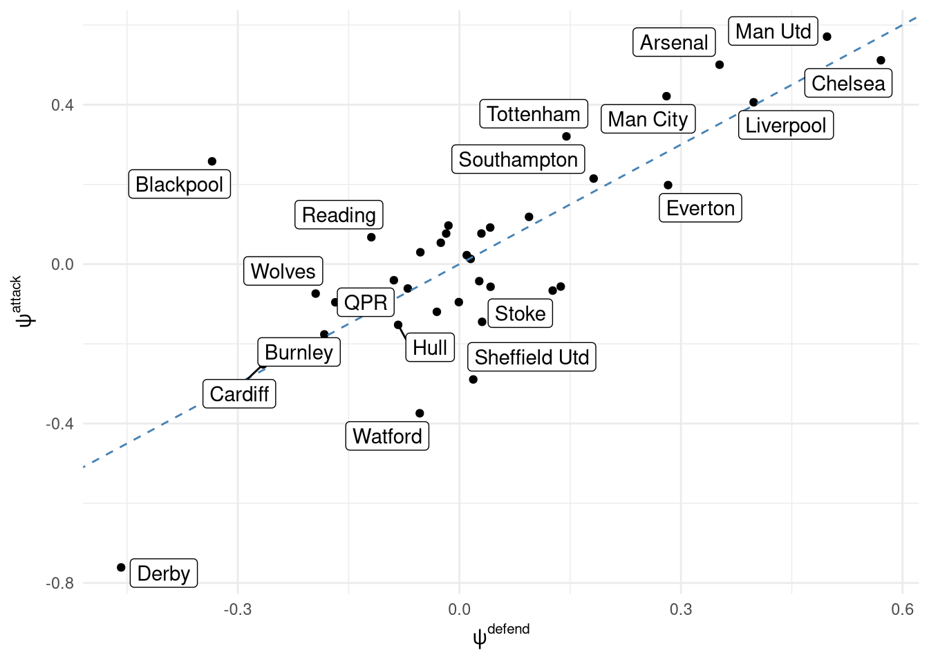
This model had 3% divergence and 0.1% max tree depth with all Rhats < 1.05 so I’ll move onto the scores, although ideally this sampling would be improved. Figure 10 shows the relationship between the 2 scores for each team, indicating a strong relationship on the whole with some outliers like Derby who are much worse at scoring goals then they are defending, or Blackpool who have a very high attacking level for their defensive record. Looking at the top-end of the table and the results align with stereotypes: Chelsea play more defensively compared to Man Utd, Arsenal, and Man City (and this is even pre-Pep).
However, the relationship between the overall skill $\psi$ from the 2 models is not what I’d expect at all, as shown in Figure 11. This is mostly because the variance in the 2-skill model is far lower: it only ranges from -0.03 to 0.02, whereas in the 1-skill model it has a range of -0.5 to 0.6. I’m unsure why this is the case, and ideally it would be fixed by modifying the priors - either the variance in the prior of the 2 skill levels or working on getting the multi-variate model sampling well as it explicitly handles the correlation. NB: Figure 10 shows that the actual $\psi^{attack}$ and $\psi^{defend}$ values themselves have a reasonable range of values - it’s just the ‘overall’ $\psi$ that doesn’t.
Figure 11: Relationship between the $\psi$ score estimated from the 1 and 2-skill models.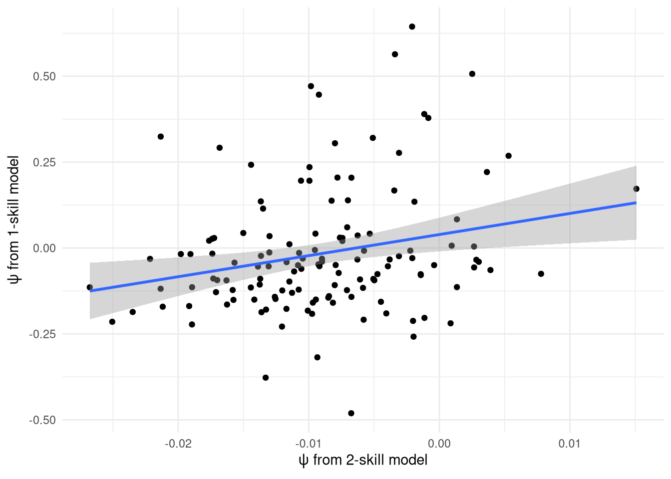
Selecting best Poisson model
To heighten up the tension I’m not going to directly compare these 3 models now - instead I’ll be doing a big comparison at the end. However, I do want to select a single Poisson model to move forwards with, so I’ll compare them on a number of metrics on the training set (it is imperative that the test set isn’t used until the final evaluation). The metrics (table below) assess the two models in 3 ways:
- On their forecasted match results (accuracy & rps)
- On the number of goals predicted (mean absolute error)
- On the model likelihood (leave-one-out cross-validation information criteria)
Fortunately the decision is easy as the 2-skill model performs best (albeit by a fine margin) on all 6 of these criteria, so it will represent a Poisson hierarchical model in the final comparison.
Show the code
predict_poisson_2 <- function(home, away, league=NULL, home_win=0, home_loss=0, away_win=0, away_loss=0, home_score=0, away_score=0, ...) {
    home_id <- match(home, training_teams)
    away_id <- match(away, training_teams)
    league_id <- match(league, leagues)
    skill_cols <- sprintf("skill[%d]", c(home_id, away_id))
    skills <- fit_pois_2$draws(skill_cols, format="draws_matrix")
    lps <- skills[, 1] - skills[, 2]
    intercept_cols <- sprintf(c("alpha_home[%d]", "alpha_away[%d]"), league_id)
    intercepts <- fit_pois_2$draws(intercept_cols, format="draws_matrix")

    # Predict home/away goals
    lp_home <- exp(intercepts[, 1] + lps)
    lp_away <- exp(intercepts[, 2] - lps)

    goals_home <- rpois(nrow(lps), lp_home)
    goals_away <- rpois(nrow(lps), lp_away)

    # Get loglik of actual home/away goals
    tibble(
        away_prob=mean(goals_away > goals_home),
        draw_prob=mean(goals_away == goals_home),
        home_prob=mean(goals_away < goals_home),
        goals_away = median(goals_away),
        goals_home = median(goals_home)
    )
}

predict_poisson_4 <- function(home, away, league=NULL, home_win=0, home_loss=0, away_win=0, away_loss=0, home_score=0, away_score=0, ...) {
    home_id <- match(home, training_teams)
    away_id <- match(away, training_teams)
    league_id <- match(league, leagues)

    if (!is.na(home_id)) {
        skill_attack_home <- fit_pois_4$draws(sprintf("skill_attack[%d]", home_id), format="draws_matrix")
        skill_defend_home <- fit_pois_4$draws(sprintf("skill_defend[%d]", home_id), format="draws_matrix")
    } else {
        # Draw random team
        skill_params <- fit_pois_4$draws(c("skill_mu", "skill_sigma"), format="draws_matrix")
        skill_overall <- rnorm(nrow(skill_params), skill_params[, 1], skill_params[, 2])
        # Draw attack and defend skills
        skill_attack_home <- rnorm(length(skill_overall), skill_overall, 2.5)
        skill_defend_home <- rnorm(length(skill_overall), skill_overall, 2.5)
    }

    if (!is.na(away_id)) {
        skill_attack_away <- fit_pois_4$draws(sprintf("skill_attack[%d]", away_id), format="draws_matrix")
        skill_defend_away <- fit_pois_4$draws(sprintf("skill_defend[%d]", away_id), format="draws_matrix")
    } else {
        # Draw random team
        skill_params <- fit_pois_4$draws(c("skill_mu", "skill_sigma"), format="draws_matrix")
        skill_overall <- rnorm(nrow(skill_params), skill_params[, 1], skill_params[, 2])
        # Draw attack and defend skills
        skill_attack_away <- rnorm(length(skill_overall), skill_overall, 2.5)
        skill_defend_away <- rnorm(length(skill_overall), skill_overall, 2.5)
    }

    intercept_cols <- sprintf(c("alpha_home[%d]", "alpha_away[%d]"), league_id)
    intercepts <- fit_pois_4$draws(intercept_cols, format="draws_matrix")

    lp_home <- exp(intercepts[, 1] + skill_attack_home - skill_defend_away)
    lp_away <- exp(intercepts[, 2] + skill_attack_away - skill_defend_home)

    # Draw predicted goals
    goals_home <- rpois(nrow(intercepts), lp_home)
    goals_away <- rpois(nrow(intercepts), lp_away)

    tibble(
        away_prob=mean(goals_away > goals_home),
        draw_prob=mean(goals_away == goals_home),
        home_prob=mean(goals_away < goals_home),
        goals_away = median(goals_away),
        goals_home = median(goals_home)
    )
}
Show the code
poisson_models <- list(
    "poisson_2"=predict_poisson_2,
    "poisson_4"=predict_poisson_4
)
Show the code
poisson_accuracy <- map_dfr(poisson_models, function(mod) {
    pmap_dfr(df |> filter(dset == "training"), mod, .progress=TRUE)
}, .id="model")
Show the code
# Calculate loo for Poisson2 model
loglik_pois2_home <- function(data_i, draws, log = TRUE) {
    lp <- exp(draws[, sprintf("alpha_home[%d]", data_i$league_id)] + draws[, sprintf("skill[%d]", data_i$home_id)] - draws[, sprintf("skill[%d]", data_i$away_id)])
    dpois(data_i$home_score, lp, log=log)
}
loglik_pois2_away <- function(data_i, draws, log = TRUE) {
    lp <- exp(draws[, sprintf("alpha_away[%d]", data_i$league_id)] + draws[, sprintf("skill[%d]", data_i$away_id)] - draws[, sprintf("skill[%d]", data_i$home_id)])
    dpois(data_i$away_score, lp, log=log)
}
Show the code
# Calculate loo for Poisson4 model
loglik_pois4_home <- function(data_i, draws, log = TRUE) {
    lp <- exp(draws[, sprintf("alpha_home[%d]", data_i$league_id)] + draws[, sprintf("skill_attack[%d]", data_i$home_id)] - draws[, sprintf("skill_defend[%d]", data_i$away_id)])
    dpois(data_i$home_score, lp, log=log)
}
loglik_pois4_away <- function(data_i, draws, log = TRUE) {
    lp <- exp(draws[, sprintf("alpha_away[%d]", data_i$league_id)] + draws[, sprintf("skill_attack[%d]", data_i$away_id)] - draws[, sprintf("skill_defend[%d]", data_i$home_id)])
    dpois(data_i$away_score, lp, log=log)
}
Show the code
# Prepare data and draws
df_train_loo <- df |>
    filter(dset == 'training') |>
    mutate(
        home_id = as.integer(factor(home, levels=training_teams)),
        away_id = as.integer(factor(away, levels=training_teams)),
        league_id = as.integer(factor(league, levels=leagues))
    )
Show the code
# Prepare draws and test function
pois2_draws <- fit_pois_2$draws(c("alpha_home", "alpha_away", "skill"), format="draws_matrix")
Show the code
# Prepare draws and test function
pois4_draws <- fit_pois_4$draws(c("alpha_home", "alpha_away", "skill_attack", "skill_defend"), format="draws_matrix")
Show the code
# Calculate r_eff
set.seed(17)
r_eff_pois2_home <- relative_eff(
    loglik_pois2_home,
    log = FALSE, # relative_eff wants likelihood not log-likelihood values
    chain_id = rep(1:4, each = 1000),
    data = df_train_loo,
    draws = pois2_draws,
    cores = 4
)
# Now calculate loo
loo_pois2_home <- loo_subsample(
    loglik_pois2_home,
    observations = 10000, # take a subsample of size 100
    cores = 4,
    # these next objects were computed above
    r_eff = r_eff_pois2_home,
    draws = pois2_draws,
    data = df_train_loo
  )

# Same for away
r_eff_pois2_away <- relative_eff(
    loglik_pois2_away,
    log = FALSE, # relative_eff wants likelihood not log-likelihood values
    chain_id = rep(1:4, each = 1000),
    data = df_train_loo,
    draws = pois2_draws,
    cores = 4
)
# Now calculate loo
loo_pois2_away <- loo_subsample(
    loglik_pois2_away,
    observations = 10000, # take a subsample of size 100
    cores = 4,
    # these next objects were computed above
    r_eff = r_eff_pois2_away,
    draws = pois2_draws,
    data = df_train_loo
  )
Show the code
# Now calculate for Poisson 4
# Calculate r_eff
set.seed(17)
r_eff_pois4_home <- relative_eff(
    loglik_pois4_home,
    log = FALSE, # relative_eff wants likelihood not log-likelihood values
    chain_id = rep(1:4, each = 1000),
    data = df_train_loo,
    draws = pois4_draws,
    cores = 4
)
# Now calculate loo
loo_pois4_home <- loo_subsample(
    loglik_pois4_home,
    observations = 10000, # take a subsample of size 100
    cores = 4,
    # these next objects were computed above
    r_eff = r_eff_pois4_home,
    draws = pois4_draws,
    data = df_train_loo
  )

# Same for away
r_eff_pois4_away <- relative_eff(
    loglik_pois4_away,
    log = FALSE, # relative_eff wants likelihood not log-likelihood values
    chain_id = rep(1:4, each = 1000),
    data = df_train_loo,
    draws = pois4_draws,
    cores = 4
)
# Now calculate loo
loo_pois4_away <- loo_subsample(
    loglik_pois4_away,
    observations = 10000, # take a subsample of size 100
    cores = 4,
    # these next objects were computed above
    r_eff = r_eff_pois4_away,
    draws = pois4_draws,
    data = df_train_loo
  )
Show the code
# Combine results
looic_pois_results <- tribble(
    ~model, ~home_looic, ~away_looic,
    "poisson_2", loo_pois2_home$estimates['looic', 1], loo_pois2_away$estimates['looic', 1],
    "poisson_4", loo_pois4_home$estimates['looic', 1], loo_pois4_away$estimates['looic', 1]
)
Show the code
rps <- function(away_prob, draw_prob, home_prob, outcome) {
    outcome_bools = rep(0, 3)
    outcome_bools[match(outcome, c('away', 'draw', 'home'))] <- 1
    probs <- c(away_prob, draw_prob, home_prob)

    0.5 * sum((cumsum(probs) - cumsum(outcome_bools))**2)
}
| Model | Accuracy (%) | RPS | Home goals | Away goals | Home goals | Away goals |
|---|---|---|---|---|---|---|
| 1-skill model | 52.7 | 0.1995 | 0.922 | 0.807 | 44123 | 39575 |
| 2-skill model | 52.8 | 0.1991 | 0.914 | 0.804 | 44086 | 39511 |