Introduction
Deep learning has attracted considerable attention for its near-human ability in a variety of complex problems such as image recognition, playing games, and recently conversational AI through large language models. Each of these applications requires unimaginable volumes of data and computational resources beyond the reach of all but the richest companies. This resource hungry nature, coupled with the huge hype that accompanies any deep-learning application, makes it challenging to gain a realistic assessment of their real-world potential for less demanding use-cases, such as scientific time-series modelling.
I was motivated to write this post because while there are a lot of tutorials for using RNNs, they nearly always had 2 very different characteristics to the type of scientific analysis I’m involved in. The first is that they tend to assume you have multiple time-series. Much like you would have multiple observations (rows) to fit a regression, some situations involve having multiple time-series so that you can treat a whole time-series as one single observation. This isn’t just a mindset only found in random blog articles, most deep learning packages seem to assume this and it can be frustrating to get around this for single univariate time-series. However, I’ll typically just have a single time-series from one location and one moment in time, or sometimes multiple time-series but all still from the same time-frame. The second difference lies in the modelling objectives. I’m mostly interested in understanding the dynamics and temporal properties of a certain pollutant, and maybe a bit of forecasting too. However, most deep learning resources I’ve seen require you to frame your problem as trying to forecast a fixed horizon ahead, using a fixed number of historical points. E.g. an overall challenge might be framed as trying to forecast 1 month sales using the previous 6 months of data, using a dataset of 1,000 different shops; a very different paradigm to the standard statistical approach of say ETS or ARIMA.
The goal of this post is to address this gap and provide an accessible and practical introduction to Neural Networks for univariate time-series analysis, and demonstrating how to do this in pytorch.
I’ll introduce the theory behind RNNs, demonstrate how to apply them to air quality datasets, discuss their advantages and disadvantages in comparison to other machine learning and statistical techniques, and provide reproducible code examples in PyTorch.
The example dataset that will be used throughout comprises hourly Ozone, Temperature and Relative Humidity measurements from the Manchester Air Quality Supersite from Jan 2020 to Jan 2021 (available from the CEDA repository), as shown in Figure 1. The objective is to predict Ozone as a function of Temperature and RH; this isn’t a scientifically interesting problem, nor is it it an especially challenging one and there is a definite ceiling to the amount of information that can be conveyed by these 2 inputs, but it provides a simple example problem.
Figure 1: Hourly dataset from Manchester supersite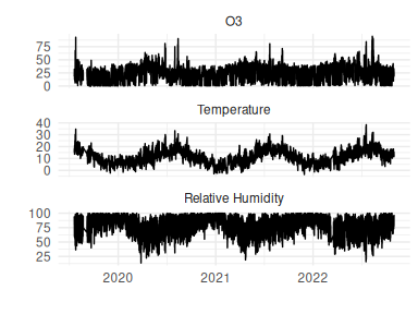
Recurrent Neural Networks
Introduction to neural networks
Before Recurrent Neural Networks are introduced, we need to mention what a standard Neural Network is, and to do that we need to discuss the fundamental building blocks: neurons. A neuron (Figure 2) is a computational unit that receives multiple inputs $X=x_1, x_2, \ldots, x_n$, multiplies them by corresponding weights $W = w_1, w_2, \ldots, w_n$, sums the products, and adds a ‘bias’ parameter $\alpha$. An activation function $f(.)$ is finally applied to obtain the output.
Figure 2: Architecture of a neuron - the building blocks of neural networks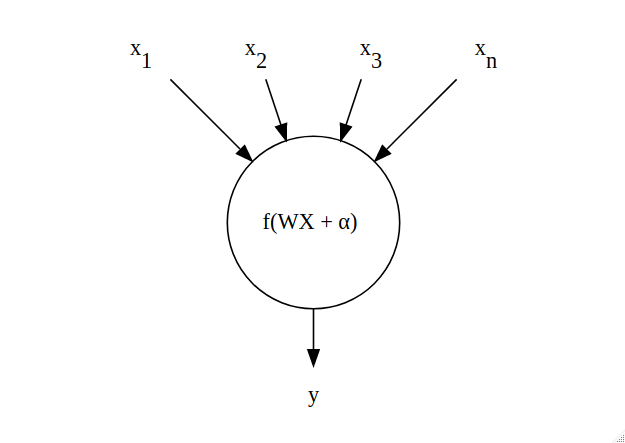
Observe that if $f(.)$ is the identity function $f(x) = x$, then a neuron is mathematically equivalent to linear regression; the weights $W$ are the same as the coefficients $\beta$ and the bias performs the same role as an intercept. Tangent: while a single neuron can be equivalent to linear regression, it is conceptually different. Linear regression specifies a probabilistic model which is estimated using maximum likelihood estimation, allowing for the provision of confidence intervals for the coefficients and prediction intervals for the outputs. Neural networks directly optimize a loss function to minimise the error between the network output and the training data, thereby only providing point estimates.
Back to the fun stuff. The function $f(.)$ facilitates a non-linear relationship between $X$ and $y$, with the 3 most popular choices shown in Figure 3 of the Sigmoid (logistic curve, $\frac{1}{1+\exp(-x)}$), Tanh, and Relu (Rectified Linear). Tanh is the only one that can output negative values, although Relu is the most commmon choice these days, owing to its ability to scale better in deeper networks.
Figure 3: Neural network activation functions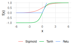
An additional way of providing non-linearity is to group multiple neurons together into hidden layers (Figure 4), allowing the network to approximate almost any non-linear function given sufficient data and training. The final layer combines the output of the previous hidden layer into a single value that is taken as the network output, $y$. This network structure is called a Multi-Layer Perceptron (MLP). It is this combination of computational units, both breadth-wise in layers and depth-wise by stacking layers, that leads to their huge success and flexibility.
Figure 4: Structure of a Multi-Layer Perceptron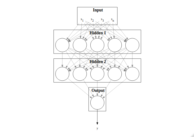
Adding memory
MLPs are great general purpose networks, but they lack one crucial property that is essential for time-series analysis: a memory. A simple way of achieving this is to pass the hidden outputs at each timestep back into the hidden layer, as shown in Figure 5, thereby allowing the neural network to combine historical knowledge about the state of the system with the new incoming data to form its predictions.
Figure 5: RNN structure for temporal inputs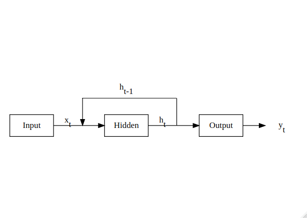
Implementation in PyTorch
Data preparation
Both the input and target variables should be transformed first, since networks expect inputs to have the bulk of their density around 0, and certainly within [-1, 1]. Transforming data into this region isn’t obligatory but it will help fitting the network weights, both in terms of speeding up the process as well as converging on more accurate estimates. Figure 6 shown the distribution of the initial example dataset under 2 different transforms: the z-score and a log-transform followed by a centering. The log-transform is preferred here as it gives a sharper normal distribution centered on 0.
Figure 6: Input data transformations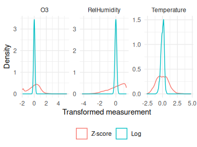
Manual implementation
The Python library pytorch was used to fit the networks themselves.
I personally found it far more user friendly than Keras/TensorFlow, not least because the lower-level API means less is abstracted, making it easier to track the flow of data around the network.
This flexibility was also particularly useful to be able to fit a model on a single time-series, similar to how a classical method such as ARIMA works.
This is in contrast to a more typical deep learning approach where you have multiple time-series and for each one you can hardcode the number of timepoints and forecast horizon, i.e. “predict the next 5 hours using the previous 48 hours of data”.
The code below shows how you would specify the RNN described in Figure 5.
The forward method is indirectly called during training with that epoch’s data and specifies the logic flow to reach the network output.
class RNNManual(nn.Module):  # Subclasses Pytorch base class
    def __init__(self, n_hidden, n_features, n_outputs):
        super(RNNManual, self).__init__()
        self.n_hidden = n_hidden
        self.n_features = n_features
        self.n_outputs = n_outputs
        # Linear is a simple neuron without an activation function
        # Note that the hidden layer accepts the number of input features + the number of hidden nodes,
        # the latter are the previous timestep's output
        self.hidden_layer = nn.Linear(n_hidden + n_features, n_hidden)
        self.hidden_activation = nn.Tanh()
        self.output_layer = nn.Linear(n_hidden, n_outputs)

    def initHidden(self):
        return torch.zeros(1, self.n_hidden)

    def forward(self, obs, previous_hidden):
        # Adds the previous hidden values as inputs to the network
        inputs = torch.cat((obs, previous_hidden), 1)
        hidden = self.hidden_layer(inputs)
        hidden_act = self.hidden_activation(hidden)
        output = self.output_layer(hidden_act)
        return output, hidden_act
The function below fits this model by iterating through each time-point and passing them into the network’s forward pass along with the previous time’s hidden activations.
The hidden states are initialised to 0 using model.initHidden() to ensure that this memory isn’t undefined at the first timestep.
The loss over the time-series is summed and used to determine the weight updates.
The process is repeated for a number of iterations known as ‘epochs’. The function returns the network, the hidden states at the end of training (so they can be used on the test set), and the loss history.
def train_manual(model, loss_function, optimizer, x, y, n_epochs):
    n_training = x.shape[0]
    losses = np.zeros(n_epochs)

    for epoch in range(n_epochs):
        model.zero_grad()  # Reset gradients
        loss = 0  # Epoch loss sum
        hidden = model.initHidden()  # Initialise hidden states to 0

        # Iterate over timepoints, getting new output predictions and accumulating loss
        for i in range(n_training):
            output, hidden = model(x[i], hidden)  # Calls 'forward' method
            loss += loss_function(output, y[i])

        loss.backward()  # Calculate the partial gradients of loss per network weight
        optimizer.step()  # Update network weights
        losses[epoch] = loss.item() / n_training

    # Return the last hidden state on the training data along with the loss history
    # and the network itself
    return model, hidden, losses
This function can be run with an initialized RNNManual instance, a loss function (here the Mean Squared Error is used although there are lots of options), and an optimization algorithm.
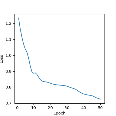
The loss quickly shrinks and then stabilizes around 15 epochs (Figure 7).
# 2 features (Temp+RH)  | 5 hidden neurons  | 1 output (Ozone)
mod_manual = RNNManual(n_hidden=5, n_features=2, n_outputs=1)
loss_func = nn.MSELoss()
# Adam is a solid optimizer to start with.
# lr = learning rate, might have to play with various values until you get a smooth loss curve
optimizer = optim.Adam(mod_manual.parameters(), lr=0.03)

mod_manual, last_hidden_manual, loss_history_manual = train_manual(mod_manual,
                                                                   loss_func,
                                                                   optimizer,
                                                                   x_train_tensor,
                                                                   y_train_tensor,
                                                                   50)
plt.clf()
plt.plot(range(1, 51), loss_history_manual)
plt.xlabel("Epoch")
plt.ylabel("Loss")
plt.show()
To get the predictions themselves, the same method of iteratively calling the network’s forward pass for each timestep is used with 1 crucial difference: torch.no_grad() is run to not accumulate gradients since we’re finished training!
Also don’t forget to convert the predictions back onto the raw measurement scale.
y_log_mean = r.means[2]

def predict_dataset_manual(data, mean, hidden=None):
    n = data.shape[0]
    preds = np.zeros(n)
    # Don't accumulate gradients since we're not training anymore
    with torch.no_grad():
        if hidden is None:
            hidden = mod_manual.initHidden()
        for i in range(n):
            pred, hidden = mod_manual(data[i], hidden)
            preds[i] = pred.item()  # Coerce vector to scalar
    # Convert predictions back to ppb
    return np.exp(preds + mean)

# On the training data the last hidden state is 0s, but on the test data
# it's the hidden state at the end of training
preds_train_manual = predict_dataset_manual(x_train_tensor, y_log_mean)
preds_test_manual = predict_dataset_manual(x_test_tensor, y_log_mean, last_hidden_manual)
This model has done relatively well at forecasting Ozone just using temperature and relative humidity, with a test set RMSE of 11.66 (Figure 8). Of course this is lower than any serious instrument, but given that it is based just off temperature and relative humidity that’s not bad! I’ve seen some commercial low-cost instruments do worse when their unreliable sensor has failed.
However, looking beyond the metrics at the actual response and the model falls short in some regards. It doesn’t fully capture the dynamics, instead having a lot more cyclical variation than the real data, which looks a lot more flat in comparison. The scatter plot shows that on average the model is under-predicting (blue line is a linear fit for the model response, pink line is a 1:1 line) with a lot of variation either side - the $R^2$ of 0.48 is nothing to write home about either. The scatter plot also shows (if you squint!) a column of points around x=0, indicating that at some times when the actual Ozone is near-zero, the prediction can get completely out-of-whack. On a ‘real’ problem this would be an interesting question to follow up.
One positive is that the model isn’t overfitting - a common concern with deep learning - this is evidenced by the network exhibiting similar behaviour on the test data as the training.
Figure 8: Predictions from manually implemented RNN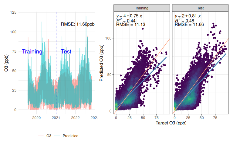
Using pytorch’s RNN layer
While the manual implementation works and is helpful to understand exactly what is going on under the hood, there is a fair amount of boiler plate code involved.
pytorch provides its own RNN layer that can be used to cut down on typing and allows the entire dataset to be passed through the network in a batch, rather than manually looping through each timestep.
This results in far more expressive code once you are familiar with the pytorch API.
For example, the forward method is now only 3 lines long vs the 5 lines from the manual class, but it doesn’t explicitly show how the recurrency is handled or what the activation function is, as that implementation detail is hidden away within the RNN layer.
NB: This network isn’t 100% identical to the manual version since the RNN layer has an additional bias term for the recurrent hidden connections, so it has 5 more free parameters.
class RNNBatch(nn.Module):
    def __init__(self, n_hidden, n_features, n_outputs):
        super(RNNBatch, self).__init__()
        self.n_hidden = n_hidden
        self.n_features = n_features
        self.n_outputs = n_outputs
        # Note the new use of a PyTorch RNN layer for the entire hidden layer
        self.hidden_layer = nn.RNN(n_features, n_hidden)
        self.output_layer = nn.Linear(n_hidden, n_outputs)

    def initHidden(self):
        # Need to add an extra dimension to the hidden layer to account for the batch dimension
        return torch.zeros(1, 1, self.n_hidden)

    def forward(self, obs, previous_hidden):
        # The forward pass is simplified as the RNN layer handles the recurrent hidden connection and the activation function
        # The output of an RNN layer is the last hidden states
        rnn_output, rnn_states = self.hidden_layer(obs, previous_hidden)
        output = self.output_layer(rnn_output)
        return output, rnn_states
The training function is also cleaner without the second loop through timestamps. This model needed a slightly higher learning rate and more epochs to fit (Figure 9) - this stage can take a bit of manual tinkering and would benefit from using a validation set to provide a more objective means of quantifying how well the training is going.
def train_batch(model, loss_function, optimizer, x, y, n_epochs):
    losses = np.zeros(n_epochs)
    for epoch in range(n_epochs):
        model.zero_grad()
        # The model can now be run in batch mode, passing an entire dataset
        # through in one go
        hidden = model.initHidden()
        output, last_hidden = model(x, hidden)
        loss = loss_function(output, y)
        loss.backward()
        optimizer.step()
        losses[epoch] = loss.item()
    return model, last_hidden, losses
mod_batch = RNNBatch(n_hidden=5, n_features=2, n_outputs=1)
loss_func = nn.MSELoss()
optimizer = optim.Adam(mod_batch.parameters(), lr=0.035)

mod_batch, last_hidden_batch, loss_history_batch = train_batch(mod_batch,
                                                               loss_func,
                                                               optimizer,
                                                               x_train_tensor,
                                                               y_train_tensor,
                                                               80)
Figure 9: Loss curve from PyTorch’s RNN implementation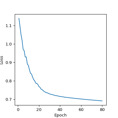
Obtaining the network’s predictions is reduced down to a single line, pruning a lot of the boilerplate code. The RMSE is very similar to the manual implementation, which is reassuring as the only difference is those extra 5 parameters (Figure 10). The network response looks better now - the predictions have more subdued extremes, although the slope is considerably lower now. It appears that this network is reducing the bias portion of the error by having a flatter response, whereas the previous network was placing greater emphasis on reducing variance by trying to capture the full dynamics (and failing).
def predict_dataset_batch(data, mean, hidden=None):
    with torch.no_grad():
        # On the training data the hidden state is initialized as zeros
        if hidden is None:
            hidden = mod_batch.initHidden()
        preds, _ = mod_batch(data, hidden)
    return np.exp((preds + y_log_mean).detach().numpy())

preds_train_batch = predict_dataset_batch(x_train_tensor, y_log_mean)
preds_test_batch = predict_dataset_batch(x_test_tensor, y_log_mean, last_hidden_batch)
Figure 10: Batch RNN predictions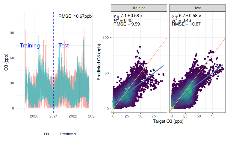
Peering into the black box
A significant limitation of machine learning techniques is that it is far harder to understand how the output predictions are being generated compared to a regression model. This section offers techniques to help shed a bit more light on neural networks’ inner workings.
Identifying non-linear relationships
With a regression model it is simple to understand how the output varies with a covariate: simply inspect its coefficient. However, with highly parameterised machine learning techniques this is not so straightforward. A simple solution is to pass in a series of known inputs and examine the effect on the output. For example, Figure 11 shows how the predicted Ozone changes with temperature at 6 evenly spaced humidities for both a linear regression and the RNN fitted above. As expected, the linear regression has a linear response with equally vertically-spaced lines of the same slope, while the RNN has both non-linear temperature responses (curves) and a non-linear RH effect (non-equally spaced lines).
Figure 11: Functional forms of a linear regression and RNN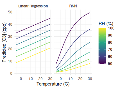
Seasonality
Atmospheric Ozone concentrations exhibit strong seasonal cycles at 3 main time-scales, as shown in Figure 12.
- Annual (peak in Spring in the Northern Hemisphere)
- Weekly (higher at weekends when NOx is lower)
- Daily (higher during daylight hours)
Figure 12: Ozone seasonal variation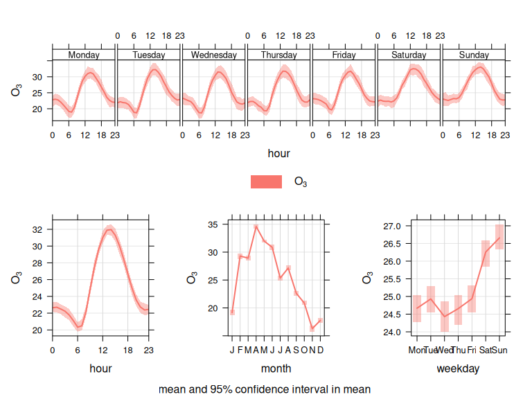
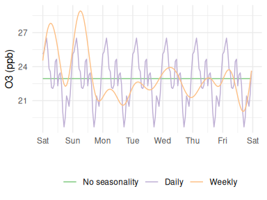
However, a result that surprised me a lot was that no matter how complex the network was, it was unable to replicate these distinctive patterns. This can be demonstrated using the same fixed-input strategy as above, but this time holding temperature and RH constant at their mean value to see if the predicted Ozone follows the expected diurnal trend. However, the network output is constant (green trace in Figure 13). On the one hand I can understand why this is the case - that if the inputs to a system are fixed then the output will be too - but I had anticipated that the RNN would be able to develop its own way of recognising these cycles.
Fortunately, seasonality can be explicitly modelled by adding dummy inputs. In particular, Fourier coefficients can be used to allow the model to form a flexible waveform at a given frequency with period $T$. $k_{max}$ is a parameter between 1 and 12 detailing how many Fourier coefficients to include and tunes the flexibility of the resultant trend: $k_{max}=1$ forms a single sine wave, while $k_{max}=12$ overfits a complex seasonal pattern. The benefit of this approach is that it doesn’t need as many parameters as the traditional dummy variable trick. I.e. modelling an annual trend with hourly data would require 8766 variables (one for each hour of the year), whereas it would only take $2k_{max}$ Fourier inputs.
$$\sin(\frac{kt2\pi}{T}), \cos(\frac{kt2\pi}{T}) \ \text{for}\ k \in 1, 2, \ldots, k_{max}$$
in this example I tried 2 networks: one with a daily trend ($T=24$) joining temperature and humidity as inputs, and one with a weekly trend ($T=168$). Of course you could add both, and even an annual trend if you had a sufficient number of full cycles in your training data. After a bit of trial-and-error I settled on $k_{max}=4$ as a good compromise between being able to pick out the dominant seasonal pattern, without adding too much additional complexity. Ideally this would be optimized through cross-validation.
Both of the new networks show the expected trends quite nicely (Figure 13). This underlies the importance of feature engineering - if it’s trivial to create an informative variable it’s generally worth doing so. With that said, I’m still intrigued how I can get the network to automatically identify these seasonal patterns for me. If anyone knows the reason for this please get in touch!
Visualizing hidden states
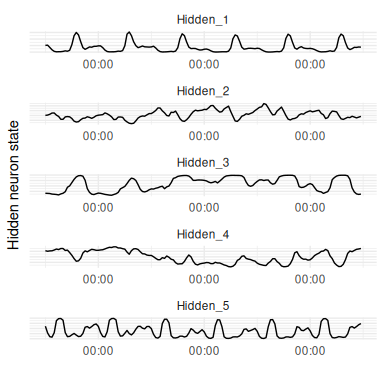
As described previously, neural networks can be thought of as automated feature construction algorithms that form non-linear representations of the data in a lower dimensionality than the input data. In an RNN these features take the form of time-dependent states. It can be instructive to look at these internal dynamics and is a simple case of storing the hidden layer outputs at each timepoint during a forward pass of the network.
The hidden states from passing 5 days of test data into the seasonal RNN shows that Hidden_1 is keeping track of the daily seasonal cycle with strong outputs just after midday, while Hidden_2 is tracking the slower O3 level (Figure 14).
Of course, for a relatively simple application such as this there is a limit to how much insight can be gained from this process since the states are largely tracking the inputs, but this property becomes more valuable the more inputs there are, the less domain knowledge there is, and where frequent interactions are expected.
Comparison with other machine learning algorithms
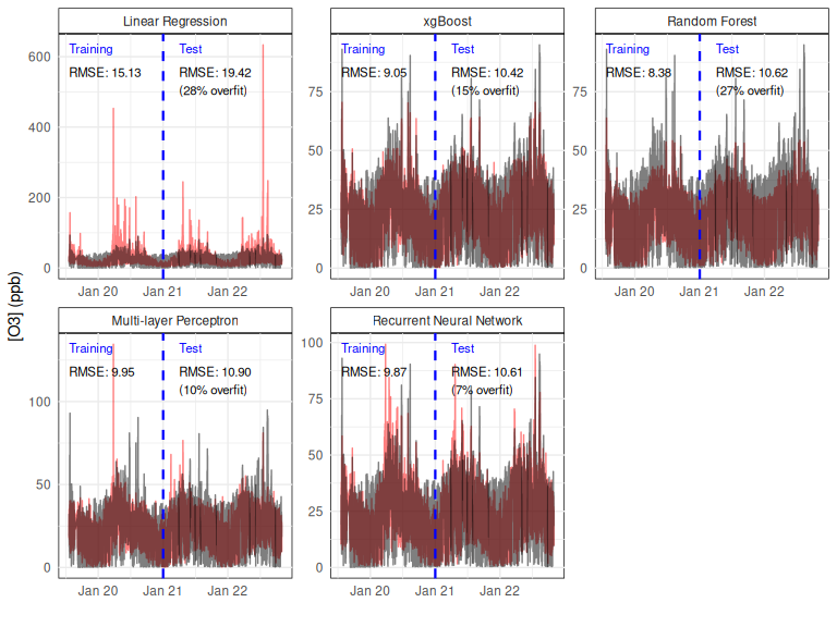
To highlight the strengths and weaknesses of RNNs when compared to other machine learning algorithms, a brief comparison has been run using the exact same dataset across 6 different statistical learning methods. In addition to the test set RMSE, the methods are evaluated on their overfitting, quantified as the percentage difference between the test and training set RMSEs. The 6 algorithms are briefly summarised below and in Table 1.
Linear Regression: standard ordinary least squares regression with none of the usual manual tweaking or diagnosticsxgBoost: One of the most popular tree-based ensemble machine learning algorithms. Hyper-parameters were selected using cross-validation over a grid-searchRandom Forest: A second tree-based algorithm. Again, hyper-parameters were tuned by a cross-validation over a grid search to hopefully reduce the tendency to overfitMulti-Layer Perceptron: The standard time-invariant Neural Network as shown in Figure 4. It had 1 hidden layer with 5 neurons and also used atanhactivation function, although no further tuning was performedRecurrent Neural Network: The same architecture as described in the previous section, with 1 hidden layer of 5 neurons. The network learning method was tweaked until the loss curve was smooth and converged within 200 epochs, but no tuning was done to optimise the architecture
| Stateful | Non-linear | |
|---|---|---|
| Linear Regression | N | N |
| xgBoost | N | Y |
| Random Forest | N | Y |
| Multi-layer Perceptron | N | Y |
| Recurrent Neural Network | Y | Y |
As shown in Figure 15, the linear regression models the mean trend well but don’t capture the full variability in Ozone concentrations.
Surprisingly, this model has the highest overfit score (% increase from training to test set).
This mostly appears due to some enormous over-predictions which go up to 600ppb in the test set; the linearity assumption has seemingly resulted in a very poor fit.
It’s less of a surprise that the next highest overfitting algorithms are the 2 tree based methods (xgBoost and Random Forests), which are known for this problem.
In a ‘real’ use case some tuning of these algorithm’s parameters would be required to reduce this.
Despite this, xgBoost actually has the best test set RMSE and random forests are second.
I imagine this is a result of the default settings for these algorithms allow for a far more highly parameterised model than my neural networks, which only have 1 hidden layer of 5 neurons (a tiny shallow network by most standards).
In spite of their small size, the neural networks achieve decent test set scores with the smallest amounts of overfitting - I’d expect increasing their size would continue to reduce the test set RMSE up until an inflexion point and overfitting starts to take over.
Having memory helps the RNN be slightly more accurate than the MLP, although given that the difference isn’t that large, I’d imagine that the greatest source of any further improvements would result from incorporating additional inputs, rather than model complexity.
