In the previous entry of what has evidently become a series on modelling
binary mixtures with Dirichlet Processes (part 1 discussed using
pymc3
and part 2 detailed writing custom Gibbs samplers), I ended by stating that I’d like to look into writing a Gibbs sampler using the stick-breaking formulation of the Dirichlet Process, in contrast to the Chinese Restaurant Process (CRP) version I’d just implemented.
Actually coding this up this was rather straight forward and took less time than I expected, but I found the differences and similarities between these two same ways of expressing the same mathematical model interesting enough for a post of its own. I’ll start by discussing the differences between these two approaches in general (for a mixture of any distribution) and then show examples specific to my case of a mixture of Bernoullis.
R package
As mentioned last time, all the code used in these posts is
available on Github as an R package
and can be installed using devtools (not tested on Windows). However, do
note that since this package is primarily written for research purposes,
it’s possible that the API used here is outdated in the future.
I do intend on cleaning it up to provide a more
consistent interface across all the samplers, as well as
refactoring the largely duplicated backend code.
For posterity, this post was written with the code at this
commit.
devtools::install_github('stulacy/bmm-mcmc')
Dataset
As with the last post, I’ll use the dataset with 1,000 observations of 5 binary variables that are formed from 3 classes. All variables have a different rate in each class - a rather nice simplification that will never occur in real world data.
library(bmmmcmc)
library(tidyverse)
data(K3_N1000_P5)
The code used to simulate this data is shown below (also available in
R/simulate_data.R).
set.seed(17)
N <- 1000
P <- 5

theta_actual <- matrix(c(0.7, 0.8, 0.2, 0.1, 0.1,
                         0.3, 0.5, 0.9, 0.8, 0.6,
                         0.1, 0.2, 0.5, 0.4, 0.9),
                       nrow=3, ncol=5, byrow = T)
cluster_ratios <- c(0.6, 0.2, 0.2)

mat_list <- lapply(seq_along(cluster_ratios), function(i) {
            n <- round(N * cluster_ratios[i])
            sapply(theta_actual[i,], function(p) rbinom(n, 1, p))
})

mat <- do.call('rbind', mat_list)
saveRDS(mat, "data/K3_N1000_P5_clean.rds")
Dirichlet Process
Let’s quickly recap Dirichlet Processes as I’ve shied away from doing it so far, mostly because I’ve only recently come to get a good feel for them myself.
The standard answer is that they are a distribution of distributions, so that each draw $G$ is in itself a distribution. Formally, they are parameterised by a base distribution $G_0$ and a concentration parameter $\alpha$.
$G \sim DP(\alpha, G_0)$
Does that make sense? If you’re like me then probably not immediately!
What helped me them really click for me was actually using them in mixture modelling, and in particular Wikipedia’s derivation of their relationship to a finite mixture model.
Starting with a standard finite mixture model, the data $y_i$ is distributed according to a known distribution $F(.)$ where each cluster has its own parameters $\theta_c$.
$$y_i\ |\ c_i,\theta \sim F(\theta_{c_i})$$
The cluster labels themselves are distributed according to a categorical distribution with probabilities given by $\pi$.
$$c_i\ |\ \pi \sim \text{Cat}_K(\pi)$$
With the prior on $\pi$ being the conjugate Dirichlet, with the concentration parameter $\alpha$.
$$\pi\ |\ \alpha \sim \text{Dirichlet}_{K}(\frac{\alpha}{K})$$
Finally, the cluster components $\theta$ are distributed according to a known distribution $G_0$.
$$\theta_c \sim G_0$$
In other words the above probability model suggests that each observation is assigned a cluster and then their data is drawn from $F$ using that cluster’s $\theta_c$. Instead, we can rewrite the same model so that it can now be thought of as each observation having their own parameter $\bar{θ}_i$.
$\bar{\theta_{i}}$ are drawn from a discrete distribution $G$, where $\delta_{\theta_k}$ is the probability distribution defined as $\delta_{\theta_k}(\theta_k) = 1$ and the probability of anything else is $0$. Thus $G$ is a distribution over probability distributions.
$$y_i\ |\ \bar{\theta}_i \sim F(\bar{\theta}_i)$$
$$\bar{\theta}_i \sim G = \sum_{k=1}^{K} \pi_k \delta_{\theta_k}(\bar{\theta}_i)$$
$$\pi\ |\ \alpha \sim \text{Dirichlet}_{K}(\frac{\alpha}{K})$$ $$\theta_c \sim G_0$$
Now, when $K$ is infinite, $G$ becomes the sum to infinity above, which is exactly how Dirichlet Process are defined, and so the model can be rewritten
$$y_i\ |\ \bar{\theta_i} \sim F(\theta_i)$$
$$\theta_i \sim G$$
$$G \sim DP(\alpha, G_0)$$
Here $G_0$ is the prior on the data parameters, for our binary data this would be the Beta distribution as the conjugate pair of the Bernoulli.
Chinese Restaurant Process
There are several alternative ways of visualising how Dirichlet Process actually work, one of the most well known being the Chinese Restaurant Process (CRP). Under this mental model, a person enters a restaurant that has a given number of tables where people are already sat (the current number of clusters in the model $K$). They either have the choice of sitting at an existing table, ideally with people they are most similar too, or sitting down at their own table.
The probability of sitting down at an existing table is given by the following, where $N_{-nc}$ is the number of people already sat at Table $c$ and $\alpha$ is a tuning parameter, where high values make it more likely that a person sets up their own table.
$$P(c_{i} = c\ |\ c_{-i}) = \frac{N_{-nc}}{N-1+\alpha}$$
The probability of sitting at a new table is given by the following, note now $α$ is on the numerator so a high value makes a new table more likely.
$$P(c_{i} = c^{*}\ |\ c_{-i}) = \frac{\alpha}{N-1+\alpha}$$
Extending these probabilities to take into account the proposed mixture model structure of the data results in Eq 3.6 of Neal (2000).
$$P(c_{i} = c\ |\ c_{-i}, y_{i}) = \frac{N_{-nc}}{N-1+\alpha}\prod_{d=1}^{D} \int F(y_i, \theta)dH_{-i, c}(\theta)$$
$$P(c_{i} = c^{*}\ |\ c_{-i}, y_{i}) = \frac{\alpha}{N-1+\alpha}\prod_{d=1}^{D} \int F(y_i, \theta)dG_{0}(\theta)$$
van der Maaten provides these integrals for the case where $F$(.) is the Bernoulli distribution, and $G_0$ is $\text{Beta}(\beta, \gamma)$.
$$P(c_{i} = c\ |\ c_{-i}, y_{i}) = \frac{N_{-nc}}{N-1+\alpha}\prod_{d=1}^{D}\frac{(\beta + \sum_{i\in C_{k}} x_{id})^{x_{nd}}(\gamma + N_{K} - \sum_{i \in C_{k}} x_{id})^{1-x_{nd}}}{\beta + \gamma + N_{k}}$$
$$P(c_{i} = c^{*}\ |\ c_{-i}, y_{i}) = \frac{\alpha}{N-1+\alpha}\prod_{d=1}^{D} \frac{B(x_{nd} + \beta, \gamma - x_{nd} +1)}{B(\beta, \gamma)}$$
These probabilities are all that is required to Gibbs sample from the Dirichlet Process Mixture Model, as $\pi$ and $\theta$ have been collapsed out (although I do add a sample step of $\alpha \sim \text{Gamma}(1, 1)$). The relative simplicity of both the required sampling steps and the conceptual model has surely helped with the popularity of the CRP as an way of explaining the Dirichlet Process.
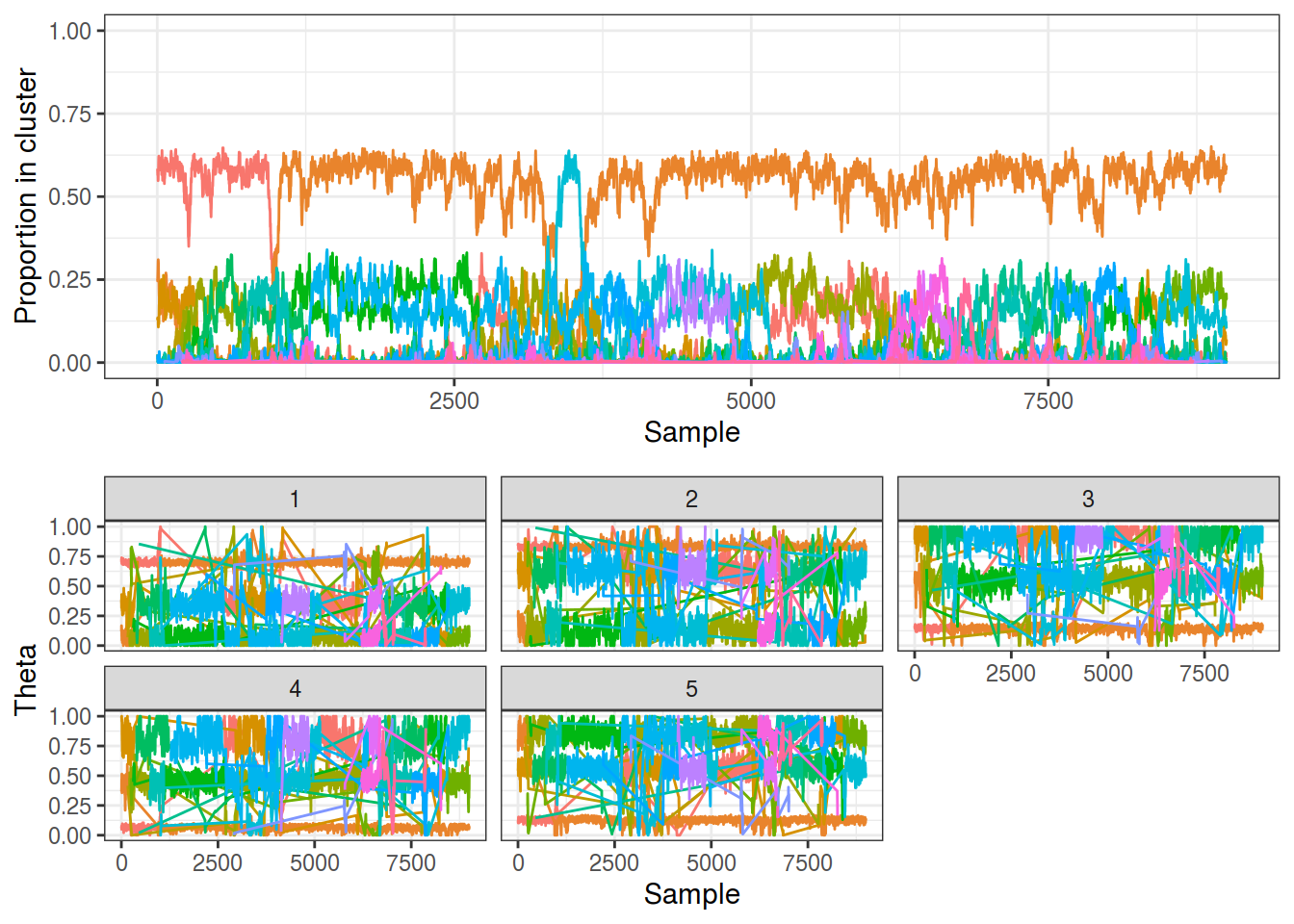
The output of my CRP sampler (code in src/collapsed_gibbs_dp.cpp) is shown below and is far more messy than the trace from a finite mixture model, even on this simple dataset. As discussed last time it suffers from the relabelling problem, although at least this means that the sampler is effectively exploring the parameter space. My particular problem is that the CRP formulation finds too many small, less supported groups, i.e. people are being assigned to sit at new tables too readily.
samp_crp <- gibbs_dp(K3_N1000_P5, nsamples = 10000, maxK = 20,
                     burnin = 1000, relabel = FALSE)
plot_gibbs(samp_crp, cluster_threshold = 0.1)

Stick-breaking
The stick breaking formulation is another perspective of how samples are drawn from a Dirichlet Process. Going back to the framing of each observation having a parameter drawn from $G$, the sum of discrete probability distributions $\delta_{\theta_k}$ over $K$:
$$\bar{\theta}_i \sim G = \sum_{k=1}^{K} \pi_k \delta_{\theta_k}(\bar{\theta}_i)$$
Sethuraman (1994) showed how the weights $\pi$ can be viewed as generated from an iterative process of breaking a stick and measuring the remaining length, where the breakpoints $V_i$ are drawn from a Beta distribution with the all-too-familiar $\alpha$ as one of the parameters.
$$\pi_i = V_{i} \prod_{j=1}^{i-1} (1 - V_{j})$$
$$V_1, \dots, V_K \sim \text{Beta}(1, \alpha)$$
Section 5.2 in Ishwaran and James (2001) provides the steps for Gibbs sampling from this method and it turns out it is rather straight forward.
Implementing the CRP sampler required ammending the finite-case collapsed Gibbs sampler by switching to data structures that can handle a flexible number of clusters, as well as modifying the cluster assignment probabilities.
The stick-breaking model on the other hand only requires a small extension to the full Gibbs sampler from the finite case, where $\pi$ are now sampled by the stick-breaking method outlined above rather than from a Dirichlet distribution, with the breakpoints generated sampled as follows.
$$V_i = \text{Beta}(1 + |c_i|, \alpha + \sum_{j=i+1}^{K-1} |c_{j}|)$$ $$V_K = 1$$
Note the use of $K$ here, which doesn’t mean the exact pre-defined number of clusters as in the finite mixture model, but instead is a maximum value so that the calculation is computationally feasible. As long as it is sufficiently larger than the expected number of different clusters in the data - Ishawaran and James (2001) note that a value of 150 for 150,000 data points was enough - the approximation will hold.
While the stick-breaking method is less obviously related to a Dirichlet Process, it is far easier to understand in terms of how to actually implement it computationally. The fact that the only difference in Gibbs sampling between the finite model and the infinite stick-breaking one is related to how how $\pi$ are sampled could explain why many people refer to the Dirichlet Process as acting as a prior on $K$, when really it is a prior on the cluster parameters themselves.
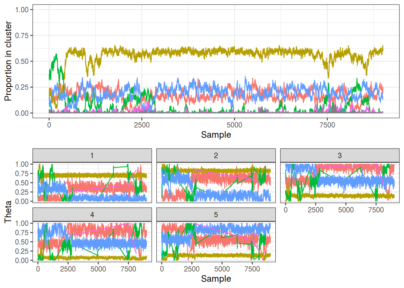
The output trace from my C++ implementation (source in src/stickbreaking.cpp) shows similar results to the CRP formulation, although there are far fewer transient groups. The reduced label switching is actually undesired behaviour since this means the sampler isn’t effectively exploring the space. This could be due to the fact the sampler is having to explore a greater space by having to sample $\theta$ and $\pi$ in addition to $z$.
samp_sb <- gibbs_stickbreaking(K3_N1000_P5, nsamples = 10000, maxK = 20,
                               burnin = 1000, relabel = FALSE)

plot_gibbs(samp_sb, cluster_threshold = 0.1)

Overall
I hope this post has provided a useful practical alternative to the very theoretical guides to Dirichlet Processes out there, and highlights implementation differences between two of the most common formulations. There has been considerable research in effectively sampling Dirichlet Processes since Ishawaran and James (2001) and Neal (2000), many of them adding jump operations in order to more effectively traverse the parameter space. However, these models are still very challenging to effectively sample from in real applications where data can be highly dimensional and multi-modal, see Hastie, Liverani, and Richardson (2015) for a thorough review.
I hope to find time to look into some of these methods, particularly the Reversible Jump MCMC (Richardson and Green 1997) and the Allocation Sampler (Nobile and Fearnside 2007) and see how applicable they are to the type of sparse high-dimensional data I typically work with.
References
Hastie, David, Silvia Liverani, and Sylvia Richardson. 2015. “Sampling from Dirichlet Process Mixture Models with Unknown Concentration Parameter: Mixing Issues in Large Data Implementations.” $Statistics and Computing$. https://doi.org/10.1007/s11222-014-9471-3.
Ishwaran, Hemant, and Lancelot James. 2001. “Gibbs Sampling Methods for Stick-Breaking Priors.” Journal of the American Statistical ASsociation. https://doi.org/10.1198/016214501750332758.
Neal, Radford. 2000. “Markov Chain Sampling Methods for Dirichlet Process Mixture Models.” Journal of Computational and Graphical Statistics. https://doi.org/10.2307/1390653.
Nobile, Agostino, and Alastair Fearnside. 2007. “Bayesian Finite Mixture Models with an Unknown Number of Components the Allocation Sampler.” Statistics and Computing. https://doi.org/10.1007/s11222-006-9014-7.
Richardson, Sylvia, and Peter Green. 1997. “On Bayesian Analysis of Mixtures with an Unknown Number of Components.” Journal of the Royal Statistical Society Statistical Methodology Series B. https://doi.org/10.1111/1467-9868.00095.
Sethuraman, Jayaram. 1994. “A constructive definition of Dirichlet Priors.” Statistica sinica.
Van Der Maaten, Laurens. n.d. “Bayesian Mixtures of Bernoulli Distributions.”