Back at the start of the year (which really doesn’t seem like that long a time ago) I was looking at using Dirichlet Processes to cluster binary data using PyMC3. I was unable to get the PyMC3 mixture model API working using the general purpose Gibbs Sampler, but after some tweaking of a custom likelihood function I got something reasonable-looking working using Variational Inference (VI). While this was still useful for exploratory analysis purposes, I’d prefer to use MCMC sampling so that I have more confidence in the groupings (since VI only approximates the posterior) in case I wanted to use these groups to generate further research questions.
After working on something else for a few months I came back to this problem with a bit more determination (and more importantly, time) and decided to try implementing my own Gibbs Sampler. I found a really useful R package called BayesBinMix that should have been ideal, since it implements several sampling methods and is specifically designed for binary data. Unfortunately, it is written in pure R and is therefore a bit too slow on the datasets I was using ($N \approx 1000$, $p \approx 50$), although others may find it suits their need.
The best remaining option then was to write my own sampler, not least so that I would have full control of how it worked and be able to tailor it to my exact specifications, but more importantly it would be a fantastic learning opportunity as I hadn’t yet coded one up, instead using general purpose libraries like PyMC3 and JAGS.
R package
Since one of my requirements was speed, I chose to write the sampler in
C++ and then build an R package around it as the Rcpp integration is
very user-friendly. All the code used in this post is available on
Github, and can be installed
using devtools (not tested on Windows):
devtools::install_github('stulacy/bmm-mcmc')
Dataset
I’ve provided several simulated datasets with this package. in this post I’ll use one with 1,000 observations of 5 binary variables that are formed from 3 classes. All variables have a different rate in each class - a rather nice simplification that will never occur in real world data.
library(bmmmcmc)
library(tidyverse)
data(K3_N1000_P5)
The code used to simulate this data is shown below (also available in
R/simulate_data.R).
set.seed(17)
N <- 1000
P <- 5

theta_actual <- matrix(c(0.7, 0.8, 0.2, 0.1, 0.1,
                         0.3, 0.5, 0.9, 0.8, 0.6,
                         0.1, 0.2, 0.5, 0.4, 0.9),
                       nrow=3, ncol=5, byrow = T)
cluster_ratios <- c(0.6, 0.2, 0.2)

mat_list <- lapply(seq_along(cluster_ratios), function(i) {
            n <- round(N * cluster_ratios[i])
            sapply(theta_actual[i,], function(p) rbinom(n, 1, p))
})

mat <- do.call('rbind', mat_list)
saveRDS(mat, "data/K3_N1000_P5_clean.rds")
Full Gibbs sampler
To get started I used a simple finite mixture model as opposed to the infinite Dirichlet Process version I used before. Where $\pi$ are cluster/component weights, $\alpha$ is a vector of concentration parameters (here $\alpha_1, \dots, \alpha_k = \frac{\alpha_0}{k}$), $z$ are the cluster labels, $\theta$ are the Bernoulli parameter which is a $k \times d$ matrix of $k$ clusters and $d$ variables, and $x$ is the data comprising an $n \times d$ binary matrix. I use the same $a$, $b$ priors on all $\theta$, here Jeffrey’s prior where $a = b = 0.5$. The concentration parameter is fixed at $\alpha_0 = 1$.
$$\pi \sim \text{Dirichlet}(\alpha_1, \dots, \alpha_k)$$
$$z \sim \text{Cat}(\pi_1, \dots, \pi_k)$$
$$θ_{kd} \sim \text{Beta}(a_{kd}, b_{kd})$$
$$x_{id} \sim \text{Bern}(\theta_{z_{i}d})$$
The first sampler I built was a full Gibbs sampler that samples from all of these random variables:
- $\pi$: The cluster weights
- $\theta$: The Bernoulli parameters (one for each cluster/variable pair)
- $z$: Cluster assignments (hard labels)
This is relatively straight forward owing to the use of conjugate priors (see Grantham’s guide here).
Since $k$ is fixed I had to assign it a value. I used $k = 3$: the known number of groups - if I couldn’t get a sampler working with a known $k$ then I had no chance when it is unknown!
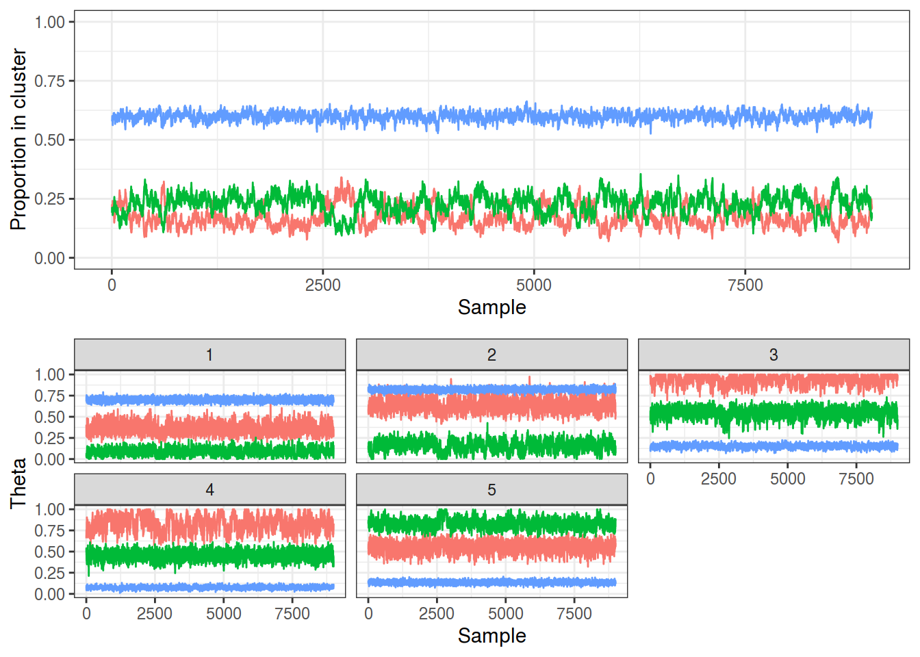
full <- gibbs_full(K3_N1000_P5, nsamples = 10000, K=3, burnin = 1000)
The traces below show a) the proportion of the dataset assigned to each of the 3 components along with b) the sampled $\theta$ values, where the line colour denotes a different component. Notice how the proportion in each cluster matches up with the 60%/20%/20% ratio I used to simulate the data, and even better, how $\theta$ match up with the known values. There is more variation in $\theta$ for the smaller two clusters as expected, and while I didn’t run any serious diagnostics, the full Gibbs sampler is able to identify the known components that generated the data for this toy problem as a proof of concept.
plot_gibbs(full)
Collapsed Gibbs
The full sampler can run into problems due to having separate values of $\theta$ for each $k$, when in reality $\theta$ may not differ too much between groups. In this instance there can be multiple observations from different groups having high probabilities of similar $\theta$ values, which then can prevent $\theta$ from updating quickly as it only updates a group at a time.
The Collapsed Gibbs sampler aims to reduce this by integrating out $\pi$ so that only the cluster labels $z$ are sampled, see Eq 3.5 in (Neal 2000) for the sampling probabilities.
$\theta$ can be estimated afterwards from the observed rates in the different components.
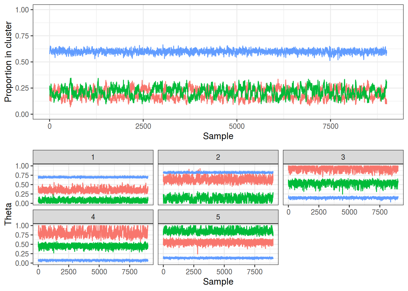
collapsed <- gibbs_collapsed(K3_N1000_P5, nsamples = 10000, K=3, burnin = 1000)
The traces below show that this sampler has also been able to identify these 3 groups with a much simpler sampling scheme.
plot_gibbs(collapsed)
Dirichlet Process
Now, while implementing these sampling methods was a valuable experience, my overall goal is to use a fully Bayesian approach where $k$ is random or even infinite.
In my tinkerings with PyMC3 I was using the stick-breaking formulation of the Dirichlet Process. However, while reading up on sampling DPs I came across a lot of literature on the Chinese Restaurant Process (CRP) and it conceptually made a lot of sense for how it extends the collapsed Gibbs sampler. In it, a new observation gets assigned either to an existing table/cluster with a probability proportional to how strongly it matches those groups (very similar to finite model), or gets assigned to a new table/cluster with a constant probability, where $\alpha$ acts as a tuning parameter for how likely new clusters are.
I implemented the CRP using Algorithm 3 from (Neal 2000). Aside from the obvious difference in that $k$ is now infinite, $\alpha$ is now a Gamma random variable with parameters $\alpha \sim \text{Gamma}(1, 1)$. For technical performance I have an argument limiting the number of clusters found, although in practice as many as the number of observations in the dataset can be found (hence this model being termed an infinite mixture model).
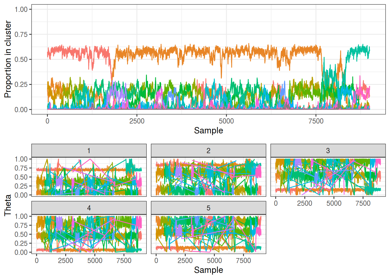
dp_1 <- gibbs_dp(K3_N1000_P5, nsamples = 10000, maxK = 20,
                 burnin = 1000, relabel = FALSE)
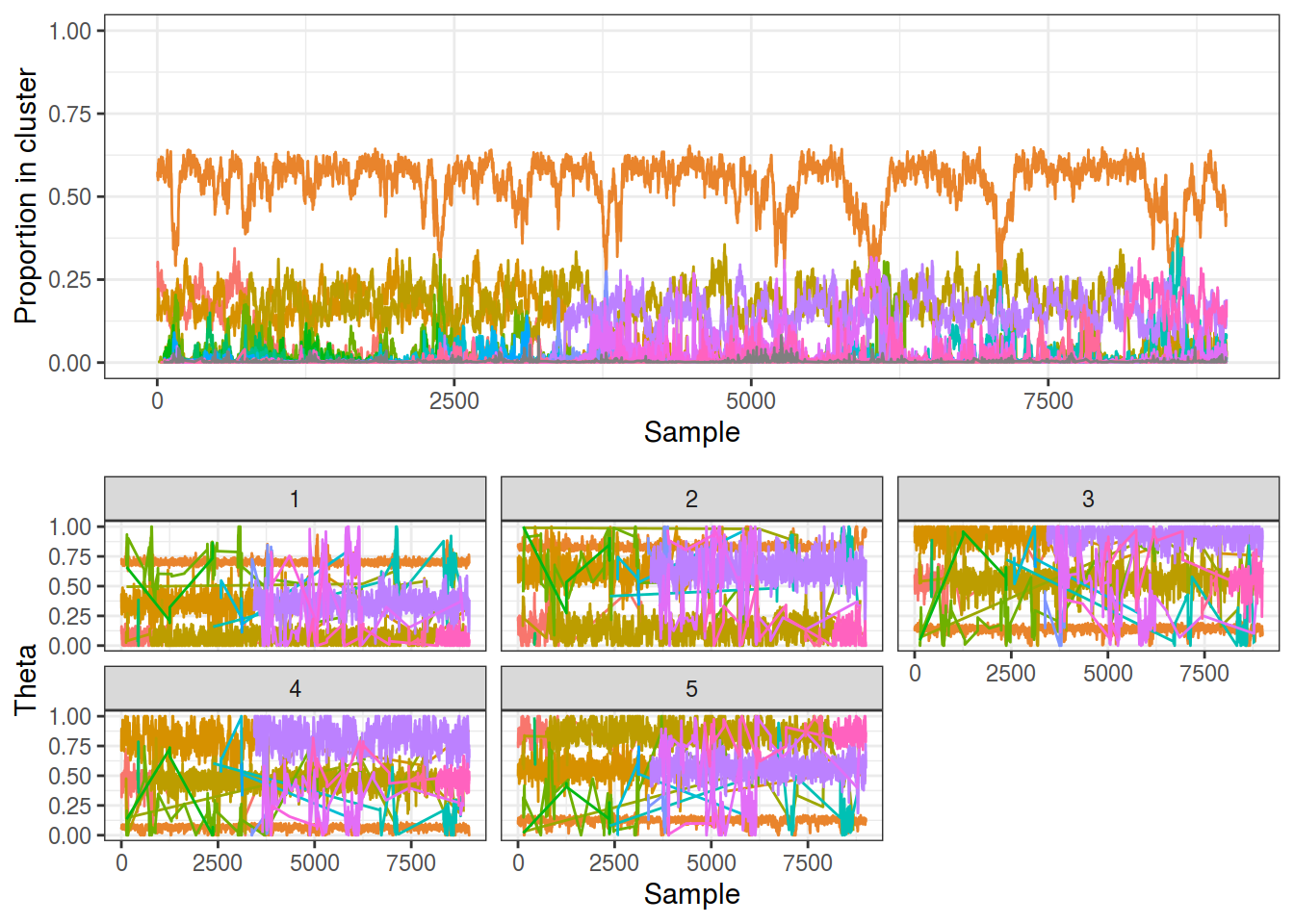
The resulting traces can be seen below, and while they are largely similar to before, there are two areas of concern:
- The traces change colour every few thousand samples! I.e. the topmost trace in the upper panel changes from red to orange to light blue
- There are a lot of components with a small number of members. Note the $\theta$ traces that drastically vary: these are from small poorly defined clusters. This is despite the plot being limited to clusters that had 10% membership at each timepoint.
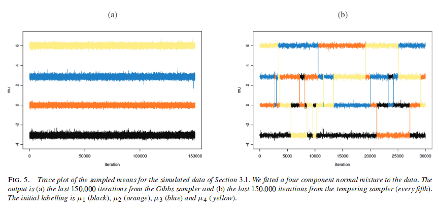
Problem 1) is what is termed the “label-switching problem”, and is actually indicative of a healthy sampler, since it means the sampler is exploring the full parameter space. Section 3.1 of (Jasra, Holmes, and Stephens 2005) details this, where Figure 5 (a) (reproduced below) is a Gibbs sampler that has only visited one of the $k!$ modes. This is the behaviour we observed in the finite sampler above, whereby it seemingly picked out the 3 groups perfectly, but in fact this demonstrated the lack of exploration. Indeed, (Jasra, Holmes, and Stephens 2005) demonstrate a modified MCMC procedure to solve this issue and as shown in Figure 5 (b) this ‘tempered Metropolis-Hastings’ method is able to move between modes, the desired behaviour.
So it’s not a bad thing that this behaviour is observed, but we’d ideally be able to obtain the original components that we know exist. Fortunately, there are various “relabelling” techniques available with this aim.
The second issue is a bit more worrying as it could indicate that alpha isn’t sampling well since lots of small poorly supported components are formed.
plot_gibbs(dp_1, cluster_threshold = 0.1)
Relabelling
I decided to focus on solving the relabelling problem first as it is commonly understood. The most well cited relabelling technique (Stephens 2000).
Again, the author of BayesBinMix has made a fantastic package called
label.switching
that performs post-hoc relabelling using a variety of methods, including
Stephen’s. However, yet again it is written in R and so is rather slow.
Furthermore, since it is post-hoc it requires storage of all cluster
assignment probabilities for every observation at every sample. For this
dataset - even if I limit the number of clusters to 20 - this is still
30,000 floats to be saved per sample, or 3e8 floats over a 10,000 sample
run. This alone uses 2GB of memory and so is unfeasible for large
datasets or for situations where the maximum number of clusters cannot
be assumed to be quite so small. Furthermore, it’s extremely slow to
run.
Fortunately, (Stephens 2000) also provides details of an online version in Section 6.2. I therefore decided to write a C++ implementation so that relabelling could be done on the fly.
Implementing the relabelling algorithm was actually the most
time-consuming part of this work, so if anyone finds it useful please
let me know. The source code is in
src/stephens.cpp
and makes use of the lpsolve Linear Programming library.
With the online relabelling method working the traces (below) look much better, although they are still not perfect. The relabeling succeeded on the most populous cluster but struggled with the 2 smaller ones - note how one group changes from orange to purple (denoting a label switch) around sample 3,5000. This isn’t a major issue as a manual relabelling would work here if needed.
This method also still suffers from the issue of small clusters appearing and disappearing rapidly, not even those with just one member but those with at least 100. This is likely due to the manner in which the Dirichlet Process works, as it is known to generate a large number of parasitic components, larger than would be found with a finite mixture model.
dp_2 <- gibbs_dp(K3_N1000_P5, nsamples = 10000, maxK = 20,
                 burnin = 1000, relabel = TRUE, burnrelabel = 500)

plot_gibbs(dp_2, cluster_threshold = 0.1)
Further Work
On the whole, implementing a custom sampler has produced far better results than using the generic PyMC3 sampler that I tried a few months ago. I’ve learnt a whole lot about Gibbs sampling and have also obtained a strong grasp of the existing literature on Bayesian Mixture Models.
There is scope for further work to take advantage of more modern sampling methods for mixture models. Firstly though I’d like to implement my own sampler for the stick-breaking formulation, just for completeness’ sake.
I’d then like to look at other ways of modelling an unknown $k$ without using the infinite $k$ approach of the Dirichlet Process. The Reversible Jump MCMC (RJMCMC) (Richardson and Green 1997) is a modified Metropolis-Hastings sampler that is designed for situations such as mixture models where the number of dimensions is unknown. On a similar note (Nobile and Fearnside 2007)’s Allocation Sampler is a more recent development of a similar idea, although it only samples from the cluster labels $z$ rather than the full joint-posterior and is therefore more efficient.
Finally, the current model I’ve been using assumes that all variables have different occurrence rates in each cluster, which is a big assumption. It’s easy to imagine a scenario where some variables aren’t differently distributed in each subgroup, or some variables that are different in one or two groups but otherwise have a general background frequency. (Elguebaly and Bouguila 2013) describes an attempt to incorporate this information into the model by using feature weighting, so each $\theta_{kd}$ has an associated Bernoulli marker which denotes whether that rate is different for that cluster to the background rate, if it isn’t then $\theta_{kd} = \theta_{d}$, thereby reducing the number of variables that impact on the clustering itself.
I’m not sure how much time I will have to work on this over the coming months but hopefully I’ll be able to post an update before too long.
References
Elguebaly, Tarek, and Nizar Bouguila. 2013. “Simultaneous Bayesian Clustering and Feature Selection Using RJMCMC-Based Learning of Finite Generalised Dirichlet Mixture Models.” Signal Processing. https://doi.org/10.1016/j.sigpro.2012.07.037.
Jasra, A, C Holmes, and D Stephens. 2005. “Markov Chain Monte Carlo Methods and the Label Switching Problem in Bayesian Mixture Modeling.” Statistical Science. https://doi.org/10.1214/088342305000000016.
Neal, Radford. 2000. “Markov Chain Sampling Methods for Dirichlet Process Mixture Models.” Journal of Computational and Graphical Statistics. https://doi.org/10.2307/1390653.
Nobile, Agostino, and Alastair Fearnside. 2007. “Bayesian Finite Mixture Models with an Unknown Number of Components the Allocation Sampler.” Statistics and Computing. https://doi.org/10.1007/s11222-006-9014-7.
Richardson, Sylvia, and Peter Green. 1997. “On Bayesian Analysis of Mixtures with an Unknown Number of Components.” Journal of the Royal Statistical Society Statistical Methodology Series B. https://doi.org/10.1111/1467-9868.00095.
Stephens, Matthew. 2000. “Dealing with Label Switching in Mixture Models.” Journal of the Royal Statistical Society Statistical Methodology Series B. https://doi.org/10.1111/1467-9868.00265.