A second post in 2 days on mixture modelling? No awards for guessing what type of analysis I’ve been preoccupied with recently!

Today’s post provides an ugly hack to fix a bug in the R flexmix package for likelihood-based mixture modelling and provides a cautionary tale about environments. In short, I’ve encountered problems when trying to predict the cluster membership for out-of-sample data using this package, and judging from a couple of posts I found online, I’m not the only one.

Simulating data

Ok let’s get to it. I’ll simulate two different datasets:

1. A mixture of 2 univariate Gaussians
2. A mixture of 2 bivariate Gaussians

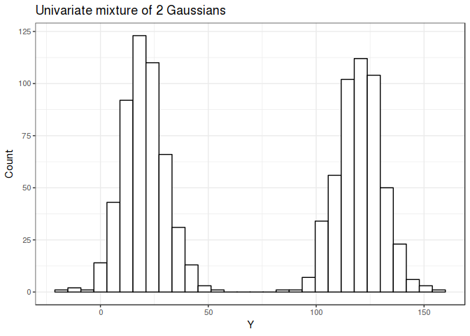
The univariate mixture is shown below with means 120 and 20, and both have a standard deviations of 10.

library(flexmix)
library(tidyverse)

N <- 1000
set.seed(17)
univariate <- rnorm(N, c(120, 20), c(10, 10))
ggplot(as.data.frame(univariate), aes(x=univariate)) +
    geom_histogram(colour='black', fill='white') +
    theme_bw() +
    labs(x="Y", y="Count", title="Univariate mixture of 2 Gaussians")

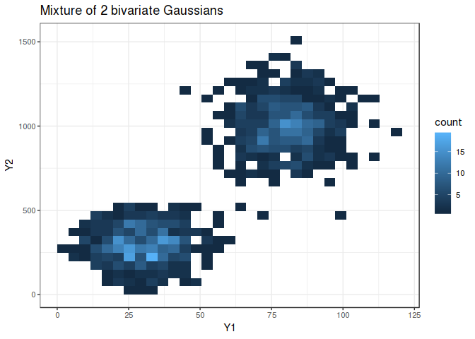
The bivariate mixture is shown below with the two groups cleanly separated (if only real world data looked like this…)

set.seed(17)
bivariate <- matrix(c(rnorm(N, c(80, 1000), c(10, 150)), 
                      rnorm(N, c(30, 300), c(10, 100))), 
                  ncol=2, byrow=TRUE)
colnames(bivariate) <- c('Y1', 'Y2')

as.data.frame(bivariate) %>%
    ggplot(aes(x=Y1, y=Y2)) +
        geom_bin2d() +
        theme_bw() +
        labs(title="Mixture of 2 bivariate Gaussians") 

Model fitting

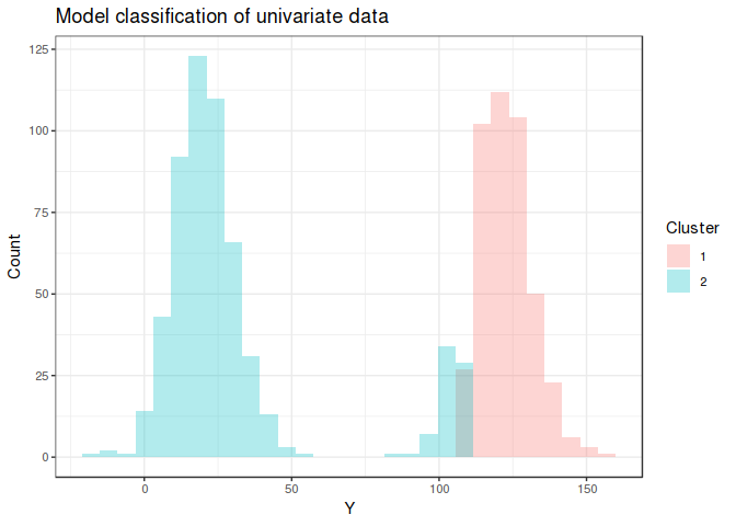
Using flexmix to fit a model with *K* = 2 for the first mixture is mostly able to distinguish the 2 underlying distributions, although I’m surprised values > 100 are included in the first group.

set.seed(17)
model_uni <- flexmix(univariate ~ 1, k = 2, control=list(iter=100),
                     model=FLXMRglm(family="gaussian"))
model_uni

## 
## Call:
## flexmix(formula = univariate ~ 1, k = 2, model = FLXMRglm(family = "gaussian"), 
##     control = list(iter = 100))
## 
## Cluster sizes:
##   1   2 
## 428 572 
## 
## convergence after 3 iterations

data.frame(univariate, cluster=model_uni@cluster) %>%
    ggplot(aes(x=univariate, fill=as.factor(cluster))) +
    geom_histogram(alpha=0.3, position='identity') +
    scale_fill_discrete("Cluster") +
    theme_bw() +
    labs(x="Y", y="Count", title="Model classification of univariate data")

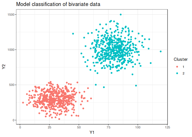
Modelling is completely successful for the somewhat easier bivariate case owing to the lack of overlap.

set.seed(17)
model_bi <- flexmix(bivariate ~ 1, k = 2, model=FLXMCmvnorm(), control=list(iter=100))
model_bi

## 
## Call:
## flexmix(formula = bivariate ~ 1, k = 2, model = FLXMCmvnorm(), 
##     control = list(iter = 100))
## 
## Cluster sizes:
##   1   2 
## 500 500 
## 
## convergence after 12 iterations

data.frame(bivariate, cluster=model_bi@cluster) %>%
    ggplot(aes(x=Y1, y=Y2, colour=as.factor(cluster))) +
    geom_point() +
    scale_colour_discrete("Cluster") +
    theme_bw() +
    labs(x="Y1", y="Y2", title="Model classification of bivariate data")

I’ll now save both these models to be used for future work in classifying as yet unseen data.

saveRDS(model_uni, "model_uni.rds")
saveRDS(model_bi, "model_bi.rds")

Classification

To simulate applying these models for new cases I’ll clear my R environment and load the models, as if we are in a production setting in a data science pipeline.

rm(list=ls())

model_uni <- readRDS("model_uni.rds")
model_bi <- readRDS("model_bi.rds")

Univariate

We’ve now received some new data, let’s see if we can predict which clusters they have arisen from. Note I’ll be attempting to predict the discrete cluster label rather than the posterior probability of each cluster, which seems relatively poorly calibrated from my initial experiments.

We have 3 samples of Y, the univariate variable, which are clear cluster 1, clear cluster 2, and a halfway point.

ndata_uni <- c(150, 20, 70)

But plugging this straight into flexmix::clusters doesn’t work as expected, seemingly because I am passing in the data as a numeric vector.

clusters(model_uni, newdata=ndata_uni)

## Error in (function (classes, fdef, mtable) : unable to find an inherited method for function 'posterior' for signature '"flexmix", "numeric"'

Let’s try wrapping it as a data frame.

ndata_uni_df <- as.data.frame(ndata_uni)
ndata_uni_df

##   ndata_uni
## 1       150
## 2        20
## 3        70

Ah that’s odd… it complains that it can’t find the variable name of the original training data…

clusters(model_uni, ndata_uni_df)

## Error in eval(predvars, data, env): object 'univariate' not found

Let’s try using this name for the data frame column.

ndata_uni_df2 <- data.frame(univariate=ndata_uni)
ndata_uni_df2

##   univariate
## 1        150
## 2         20
## 3         70

And there we go, and it gets the predictions correct and predicts the midway point as cluster 2, which we’d expect from the histogram.

clusters(model_uni, ndata_uni_df2)

## [1] 1 2 2

NB: what I mean about “poorly calibrated posteriors” is shown below, where there is a <1% posterior difference for all 3 points.

posterior(model_uni, ndata_uni_df2)

##           [,1]      [,2]
## [1,] 0.5042937 0.4957063
## [2,] 0.4908194 0.5091806
## [3,] 0.4959340 0.5040660

Bivariate

Now let’s do the same for the bivariate case, these new measurements should be assigned to cluster 2 which had means of 80 and 1000.

ndata_bi <- c(80, 1000)

Again, we get the error about not being able to pass vectors into clusters.

clusters(model_bi, newdata=ndata_bi)

## Error in (function (classes, fdef, mtable) : unable to find an inherited method for function 'posterior' for signature '"flexmix", "numeric"'

Again trying to pass the values in as a data frame results in an error message that it cannot find the bivariate variable.

ndata_bi_df <- data.frame(y1=80, y2=1000)
clusters(model_bi, newdata=ndata_bi_df)

## Error in eval(predvars, data, env): object 'bivariate' not found

The solution for the univariate case was to pass in a data frame where the column had the name of the original matrix, but obviously this won’t work here. Perhaps calling this data frame the same as the original training data will do the trick?

Nope, this still fails.

bivariate <- data.frame(Y1=80, Y2=1000)
clusters(model_bi, newdata=bivariate)

## Error in model.frame.default(model@terms, data = data, na.action = NULL, : invalid type (list) for variable 'bivariate'

Solution

After a while of tearing my hair out, I managed to fix this with a particularly beautiful hack, shown below.

Essentially, the code needs a variable with the same name and data type as the original training data (bivariate in this case and a matrix). It uses eval to run the prediction, which looks for this variable in the current environment, hence the use of the <-- operator, which assigns this name in the global environment.

The other point to note is that the newdata keyword is expecting a data frame, not a matrix, so we must pass it such. However, it never actually uses the passed in value, so as long as this is a data frame with the same number of rows as the actual data it doesn’t matter what the values are.

predict_cluster <- function(y1, y2) {
    bivariate <<- matrix(c(y1, y2), ncol=2)
    clusters(model_bi, newdata=data.frame(dummy=rep(1, length(y1))))
}

This function now correctly classifies the means of the two distributions.

predict_cluster(80, 1000)

## [1] 2

predict_cluster(30, 300)

## [1] 1

And by setting the dummy data frame length, it can be used for arbitrary length input.

predict_cluster(c(80, 30, 50), c(1000, 300, 500))

## [1] 2 1 1

That’s it for today, the lesson being take extreme care when using eval in your code and to setup a high coverage testing suite. Development of the package looks to have gone stale, and the source code isn’t on GitHub else I would have submitted this fix as a PR. Please let me know if you’ve also encountered this issue and this post has helped!