I’ve recently expanded my hierarchical Bayesian football (aka soccer) prediction football prediction framework to predict the results of Australian Rules Football (AFL) matches. I have no personal interest in AFL, instead I got involved through an email sent to a statistics mailing list advertising a competition that’s held by Monash University in Melbourne. Sensing an opportunity to quickly adapt my soccer prediction method to AFL results and to compare my technique to others, I decided to get involved.
I should note that throughout this competition I haven’t spent significant time on tailoring my Predictaball model to the new task of AFL prediction, instead I’m quite happy to spend the 5 minutes a week of updating last week’s results and obtaining this week’s predictions. I haven’t sought out any additional data aside from that which is provided by the competition organisers, which consists of historical scores going back to 1998, as well as bookies odds - the latter I don’t use at all.
Data
I first grab the historical training data from an SQLite DB I setup for this project.
As with Predictaball, I quantify each team’s recent form by their number of wins in recent games. For the AFL prediction I’m currently using the last 3 games to measure form, but once 5 rounds have been played I’ll increase this up to 5.
Note that the aim of this competition isn’t to provide probabilities of all 3 outcomes (home win, away win, draw), but rather to estimate the probability of the home team winning. As a result, I create a new dummy target variable as a binary value of whether the home team won or not. If I was interested in predicting all 3 outcomes (as I am with Predictaball), then I’d use an ordered logit regression, but this simplification allows us to model the outcome as being binomially distributed.
# sel_data is the data frame containing results extracted from my DB
sel_data$outcome2 <- factor(sel_data$outcome == 'h', labels=c('n', 'y'))
head(sel_data)
    ##          home       away hwon hdrawn hlost awon adrawn alost outcome
    ## 1    St_Kilda  Fremantle    2      0     1    2      0     1       a
    ## 2     Carlton   Essendon    3      0     0    3      0     0       a
    ## 3 Collingwood P_Adelaide    1      0     2    1      0     2       h
    ## 4    Adelaide G_W_Sydney    2      0     1    0      0     3       h
    ## 5    Brisbane Gold_Coast    1      0     2    0      0     3       h
    ## 6     W_Coast   Hawthorn    3      0     0    2      0     1       h
    ##   season outcome2
    ## 1   2012        n
    ## 2   2012        n
    ## 3   2012        y
    ## 4   2012        y
    ## 5   2012        y
    ## 6   2012        y
Due to the long time taken to fit a Bayesian model, I can’t feasibly run cross-validation for either model selection or evaluation. For model selection this isn’t an issue since I’m being lazy and just building a very similar functional form to that which I currently use for soccer prediction. For model evaluation this isn’t a major concern either as the model will get assessed at the end of each week automatically by the competition organisers.
To obtain an idea of how well my models are fitting, I’ll use a single holdout set, taken as the most recent season. I’ll use all the other 18 seasons for fitting the model.
train_df <- sel_data %>%
                filter(season != 2016) %>%
                dplyr::select(-season)
test_df <- sel_data %>%
                filter(season == 2016) %>%
                dplyr::select(-season)
head(train_df)
    ##          home       away hwon hdrawn hlost awon adrawn alost outcome
    ## 1    St_Kilda  Fremantle    2      0     1    2      0     1       a
    ## 2     Carlton   Essendon    3      0     0    3      0     0       a
    ## 3 Collingwood P_Adelaide    1      0     2    1      0     2       h
    ## 4    Adelaide G_W_Sydney    2      0     1    0      0     3       h
    ## 5    Brisbane Gold_Coast    1      0     2    0      0     3       h
    ## 6     W_Coast   Hawthorn    3      0     0    2      0     1       h
    ##   outcome2
    ## 1        n
    ## 2        n
    ## 3        y
    ## 4        y
    ## 5        y
    ## 6        y
The proportion of home wins is:
table(train_df$outcome2) / nrow(train_df) * 100
##        n        y
## 41.90412 58.09588
So we really want to beat 60% to obtain a useful model.
Benchmark models
In the previous section I stated that I wouldn’t be performing any model
evaluation. This isn’t entirely true, as I’ll compare the fully Bayesian
model to a Naive Bayes classifier that can train in a fraction (seconds
rather than an hour) of the time needed. I’ll also use an xgBoost
implementation for a more complex, but still quicker to fit, model.
These benchmark models will be rather naive models, only provided each
team’s form, rather than any measure of team strength. Thus it would be
assumed the fully Bayesian model will be more accurate. Also note that
again I’m being lazy and just using the default caret tuning grid for
these learning algorithms.
For these benchmark classifiers, I’ll use a basic caret training procedure with repeated cross-validation and the log-loss cost function.
tr <- trainControl(method='repeatedcv',
                   number=10,
                   repeats=5,
                   classProbs=T,
                   summaryFunction=mnLogLoss
                   )
Naive Bayes
The Naive Bayes classifier fits in seconds.
set.seed(3)
nb <- train(outcome2 ~ hwon + awon,
            method='nb',
            metric='logLoss',
            trControl=tr,
            data=train_df)
nb
## Naive Bayes
##
## 2983 samples
##    2 predictors
##    2 classes: 'n', 'y'
##
## No pre-processing
## Resampling: Cross-Validated (10 fold, repeated 5 times)
## Summary of sample sizes: 2685, 2685, 2685, 2685, 2685, 2684, ...
## Resampling results across tuning parameters:
##
##   usekernel  logLoss
##   FALSE      0.6407220
##    TRUE      0.6521055
##
## Tuning parameter 'fL' was held constant at a value of 0
## Tuning
##  parameter 'adjust' was held constant at a value of 1
## logLoss was used to select the optimal model using  the smallest value.
## The final values used for the model were fL = 0, usekernel = FALSE
##  and adjust = 1.
While the log-loss is a useful cost measure for classification tasks, it is not that interpretable; what does a log-loss value of 0.64 actually mean? It’ll be useful to compare it to other models but on its own it doesn’t allow for an intuitive appreciation of model fit.
min(nb$results$logLoss)
## [1] 0.640722
This is where it can be useful to obtain the model’s accuracy to obtain an idea of how much practical relevance the model has. This model’s accuracy on its training set is 62%, as shown below, which isn’t amazing considering the oracle accuracy is 60%, but isn’t too bad when considering the only inputs to this classifier are the last three results.
mean(predict(nb, newdata=train_df) == train_df$outcome2)
## [1] 0.6221924
xgBoost
Let’s see if a state-of-the-art machine learning algorithm can do any better than the naive bayes. Also note that we can provide the home and away team here since tree-based methods can handle low-variance categorical data far better than the Naive Bayes (which wouldn’t converge with these factors). However, note that this isn’t a hierarchical model, i.e. the xgBoost tree doesn’t recognise that the value of Sydney as a home team is the same team as the Sydney in the away team input.
set.seed(3)
xgb <- train(outcome2 ~ home + away + hwon + awon,
             data=train_df,
             metric='logLoss',
             trControl=tr,
             method='xgbTree')
xgb
## eXtreme Gradient Boosting
##
## 2983 samples
##    4 predictors
##    2 classes: 'n', 'y'
##
## No pre-processing
## Resampling: Cross-Validated (10 fold, repeated 5 times)
## Summary of sample sizes: 2685, 2685, 2685, 2685, 2685, 2684, ...
## Resampling results across tuning parameters:
##
##   eta  max_depth  colsample_bytree  subsample  nrounds  logLoss
##   0.3  1          0.6               0.50        50      0.6340194
##   0.3  1          0.6               0.50       100      0.6341923
##   0.3  1          0.6               0.50       150      0.6339301
##   0.3  1          0.6               0.75        50      0.6332515
##   0.3  1          0.6               0.75       100      0.6327496
##   0.3  1          0.6               0.75       150      0.6331829
##   0.3  1          0.6               1.00        50      0.6343153
##   0.3  1          0.6               1.00       100      0.6317279
##   0.3  1          0.6               1.00       150      0.6316498
##   0.3  1          0.8               0.50        50      0.6340190
##   0.3  1          0.8               0.50       100      0.6348201
##   0.3  1          0.8               0.50       150      0.6350264
##   0.3  1          0.8               0.75        50      0.6332341
##   0.3  1          0.8               0.75       100      0.6327092
##   0.3  1          0.8               0.75       150      0.6336241
##   0.3  1          0.8               1.00        50      0.6342879
##   0.3  1          0.8               1.00       100      0.6316945
##   0.3  1          0.8               1.00       150      0.6316395
##   0.3  2          0.6               0.50        50      0.6352954
##   0.3  2          0.6               0.50       100      0.6380391
##   0.3  2          0.6               0.50       150      0.6410072
##   0.3  2          0.6               0.75        50      0.6325316
##   0.3  2          0.6               0.75       100      0.6369984
##   0.3  2          0.6               0.75       150      0.6411875
##   0.3  2          0.6               1.00        50      0.6323639
##   0.3  2          0.6               1.00       100      0.6363287
##   0.3  2          0.6               1.00       150      0.6402175
##   0.3  2          0.8               0.50        50      0.6358888
##   0.3  2          0.8               0.50       100      0.6392647
##   0.3  2          0.8               0.50       150      0.6431819
##   0.3  2          0.8               0.75        50      0.6338695
##   0.3  2          0.8               0.75       100      0.6378576
##   0.3  2          0.8               0.75       150      0.6420315
##   0.3  2          0.8               1.00        50      0.6322382
##   0.3  2          0.8               1.00       100      0.6361102
##   0.3  2          0.8               1.00       150      0.6398716
##   0.3  3          0.6               0.50        50      0.6394713
##   0.3  3          0.6               0.50       100      0.6471032
##   0.3  3          0.6               0.50       150      0.6544207
##   0.3  3          0.6               0.75        50      0.6369555
##   0.3  3          0.6               0.75       100      0.6479796
##   0.3  3          0.6               0.75       150      0.6564616
##   0.3  3          0.6               1.00        50      0.6370824
##   0.3  3          0.6               1.00       100      0.6473225
##   0.3  3          0.6               1.00       150      0.6553860
##   0.3  3          0.8               0.50        50      0.6426640
##   0.3  3          0.8               0.50       100      0.6514799
##   0.3  3          0.8               0.50       150      0.6617544
##   0.3  3          0.8               0.75        50      0.6398737
##   0.3  3          0.8               0.75       100      0.6505461
##   0.3  3          0.8               0.75       150      0.6598278
##   0.3  3          0.8               1.00        50      0.6375502
##   0.3  3          0.8               1.00       100      0.6478913
##   0.3  3          0.8               1.00       150      0.6571539
##   0.4  1          0.6               0.50        50      0.6339718
##   0.4  1          0.6               0.50       100      0.6354407
##   0.4  1          0.6               0.50       150      0.6349708
##   0.4  1          0.6               0.75        50      0.6331067
##   0.4  1          0.6               0.75       100      0.6337126
##   0.4  1          0.6               0.75       150      0.6341673
##   0.4  1          0.6               1.00        50      0.6328334
##   0.4  1          0.6               1.00       100      0.6316159
##   0.4  1          0.6               1.00       150      0.6320620
##   0.4  1          0.8               0.50        50      0.6337016
##   0.4  1          0.8               0.50       100      0.6340724
##   0.4  1          0.8               0.50       150      0.6341252
##   0.4  1          0.8               0.75        50      0.6327357
##   0.4  1          0.8               0.75       100      0.6338157
##   0.4  1          0.8               0.75       150      0.6341898
##   0.4  1          0.8               1.00        50      0.6328583
##   0.4  1          0.8               1.00       100      0.6315859
##   0.4  1          0.8               1.00       150      0.6320476
##   0.4  2          0.6               0.50        50      0.6364542
##   0.4  2          0.6               0.50       100      0.6398969
##   0.4  2          0.6               0.50       150      0.6452034
##   0.4  2          0.6               0.75        50      0.6357187
##   0.4  2          0.6               0.75       100      0.6404164
##   0.4  2          0.6               0.75       150      0.6458445
##   0.4  2          0.6               1.00        50      0.6340203
##   0.4  2          0.6               1.00       100      0.6395627
##   0.4  2          0.6               1.00       150      0.6437687
##   0.4  2          0.8               0.50        50      0.6384505
##   0.4  2          0.8               0.50       100      0.6435016
##   0.4  2          0.8               0.50       150      0.6485120
##   0.4  2          0.8               0.75        50      0.6371693
##   0.4  2          0.8               0.75       100      0.6432734
##   0.4  2          0.8               0.75       150      0.6478184
##   0.4  2          0.8               1.00        50      0.6343541
##   0.4  2          0.8               1.00       100      0.6402530
##   0.4  2          0.8               1.00       150      0.6450308
##   0.4  3          0.6               0.50        50      0.6447538
##   0.4  3          0.6               0.50       100      0.6598096
##   0.4  3          0.6               0.50       150      0.6694833
##   0.4  3          0.6               0.75        50      0.6431007
##   0.4  3          0.6               0.75       100      0.6569459
##   0.4  3          0.6               0.75       150      0.6699318
##   0.4  3          0.6               1.00        50      0.6401776
##   0.4  3          0.6               1.00       100      0.6541456
##   0.4  3          0.6               1.00       150      0.6640595
##   0.4  3          0.8               0.50        50      0.6471922
##   0.4  3          0.8               0.50       100      0.6634678
##   0.4  3          0.8               0.50       150      0.6748524
##   0.4  3          0.8               0.75        50      0.6458011
##   0.4  3          0.8               0.75       100      0.6607604
##   0.4  3          0.8               0.75       150      0.6734770
##   0.4  3          0.8               1.00        50      0.6419818
##   0.4  3          0.8               1.00       100      0.6560187
##   0.4  3          0.8               1.00       150      0.6670558
##
## Tuning parameter 'gamma' was held constant at a value of 0
##
## Tuning parameter 'min_child_weight' was held constant at a value of 1
## logLoss was used to select the optimal model using  the smallest value.
## The final values used for the model were nrounds = 100, max_depth = 1,
##  eta = 0.4, gamma = 0, colsample_bytree = 0.8, min_child_weight = 1
##  and subsample = 1.
The xgBoost model has a lower log-loss (0.63 to 0.64) than the naive bayes, but this could be expected owing to the more complex model with a larger number of paramters. Does this difference have any significant impact on the model’s ability to accurately predict the outcome of future AFL matches?
min(xgb$results$logLoss)
## [1] 0.6315859
As with the Naive Bayes model, the training set accuracy is calculated. 65% is actually a fair bit better than the Naive Bayes score of 62%, which is interesting as their logloss wasn’t that different.
mean(predict(xgb, newdata=train_df) == train_df$outcome2)
## [1] 0.6526986
Overall then, not a drastically brilliant performance from either xgBoost or the Naive Bayes model. Perhaps there is simply not sufficient information available in the form predictors I use to accurately predict matches. As I’m not personally overly interested in AFL results, and owing to the time-constraints of the already-underway Monash competition, I’m not willing to obtain additional information to help improve this model. Maybe providing a hierarchical model with an input corresponding to team strength will help, as demonstrated by the fully Bayesian model.
Hierarchical Bayesian Model
Model definition
The model itself is a rather simple hierarchical model with a logit link since we have a binary outcome. We model the logit probability of a home win as the linear predictor of the inputs, i.e.:
$$logit(p_{i})=\alpha + skill_{home} − skill_{away} + \beta z_{i}$$
Where $z$ is a vector comprising:
- $hw$: The number of wins from the home team in the last 3 matches
- $aw$: The number of wins from the away team in the last 3 matches
Note that this hierarchical model has two levels, one is the individual match level predictors, for which we have form for both the away and home team, and a team level model, which currently consists of intercepts for both teams. The predictors in this instance are actually team-level variables; better examples of match-level inputs would include date, temperature, and stadium.
Unlike the xgBoost classifier, the fully Bayesian model will assign a single skill value for each team, no matter whether they are home or away. This allows for a simpler model that in theory should be able to better capture any trends. of course this model assumes that each team’s skill is independent of whether they are home or away, and the difference between a team’s home and away skill is always the same and can be represented by $\alpha$.
m_string <- "model {
for (i in 1:ngames) {
    # Linear predictor. Now need to obtain probability as logit of LP
    mu[i] <- alpha + skill[hometeam[i]] - skill[awayteam[i]] + beta_hw * homewin[i] + beta_aw * awaywin[i]

    logit(p[i]) <- mu[i]
    result[i] ~ dbern(p[i])
}

    # Priors over coefficients
    alpha ~ dnorm(0, 1.0E-3)
    beta_hw ~ dnorm(0, 1.0E-3)
    beta_aw ~ dnorm(0, 1.0E-3)

    # Prior for skill, with 0 as baseline
    skill[1] <- 0
    for(j in 2:nteams) {
        skill[j] ~ dnorm(group_skill, group_tau)
    }

    # Note that the skill variance was listed as 16, but here need the reciprocal
    # as JAGS uses tau
    group_skill ~ dnorm(0, 0.0625)
    group_tau <- 1 / pow(group_sigma, 2)
    group_sigma ~ dunif(0, 3)
}"
teams <- unique(c(train_df$home, train_df$away))
JAGS requires a list of the data inputs for the model, this is where the continuous covariates are scaled to aid convergence.
# Pass data into model
data_list <- list(result = as.numeric(train_df$outcome2)-1,
                  hometeam = as.numeric(factor(train_df$home,
                                               levels=teams)),
                  awayteam = as.numeric(factor(train_df$away,
                                               levels=teams)),
                  homewin = train_df$hwon - mean(train_df$hwon),
                  awaywin = train_df$awon - mean(train_df$awon),
                  ngames = nrow(train_df),
                  nteams = length(teams)
                 )
The final thing we need to help convergence is some initial estimates for the coefficients, which can be easily provided with a maximum likelihood estimate of the form factors:
lr <- glm(outcome2 ~ hwon + awon, data=train_df, family = binomial(link='logit'))
lr
##
## Call:  glm(formula = outcome2 ~ hwon + awon, family = binomial(link = "logit"),
##     data = train_df)
##
## Coefficients:
## (Intercept)         hwon         awon
##      0.2296       0.5008      -0.3925
##
## Degrees of Freedom: 2982 Total (i.e. Null);  2980 Residual
## Null Deviance:       4057
## Residual Deviance: 3821  AIC: 3827
As expected, winning previous games has a positive impact on the probability of a home win, increasing the log-odds by 0.5. Unsurprisingly, the away team winning recent games has a negative impact on the home team’s chances.
The intercept provides the home-win probability when both teams are at average form, which is:
1 / (1 + exp(-0.2296))
## [1] 0.5571492
This is slightly lower than the 58% as indicated on the training set but again highlights the home advantage.
table(train_df$outcome2) / nrow(train_df)
##
##         n         y
## 0.4190412 0.5809588
Model Fitting
I’ll build this model using a relatively large number of iterations since it doesn’t take comparatively too long (~20 mins).
m <- jags.model(textConnection(m_string), data=data_list,
                inits=list(beta_hw=coef(lr)['hwon'],
                           beta_aw=coef(lr)['awon']),
                n.chains=3, n.adapt=10000)
## Compiling model graph
##    Resolving undeclared variables
##    Allocating nodes
## Graph information:
##    Observed stochastic nodes: 2983
##    Unobserved stochastic nodes: 22
##    Total graph size: 19408
##
## Initializing model
Need to run some burn-in too, again can use a rather large value here since this process doesn’t take too long.
update(m, 10000)
The final step in using JAGS is to actually obtain our samples from the posterior.
s <- coda.samples(m, variable.names = c("alpha", "skill", "group_skill", "group_sigma", "beta_hw", "beta_aw"),
                  n.iter=10000, thin=2)
plot(s)
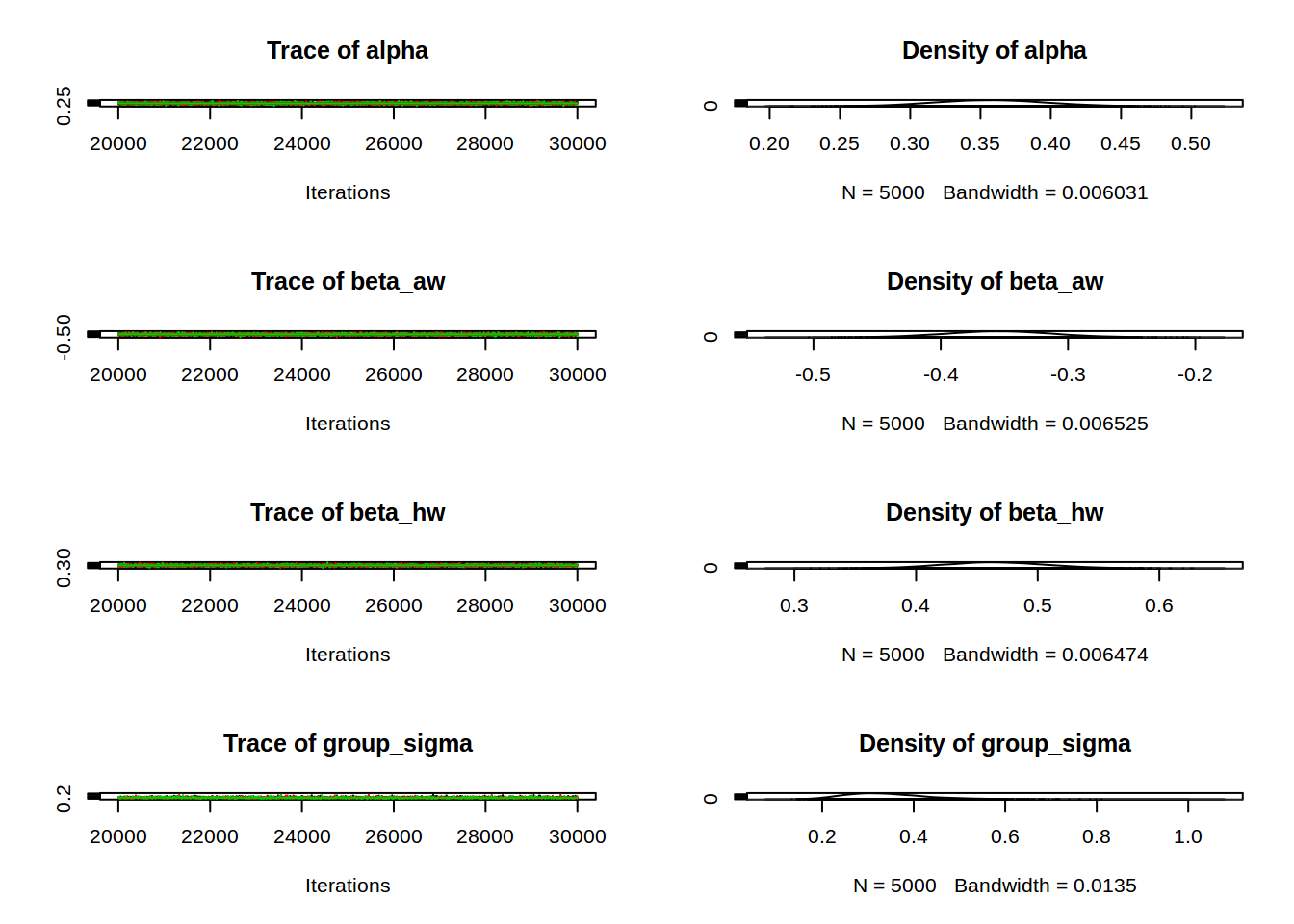
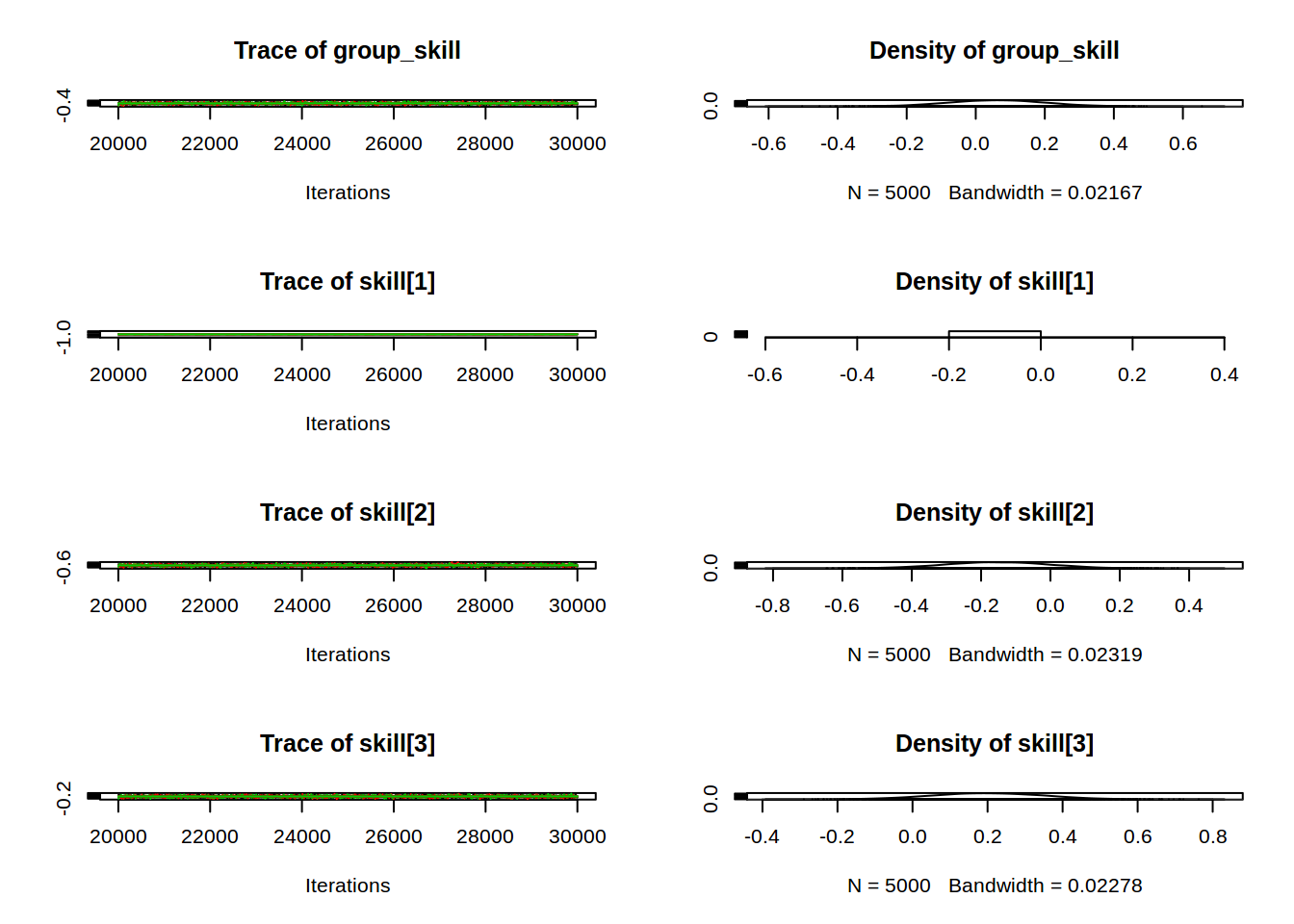
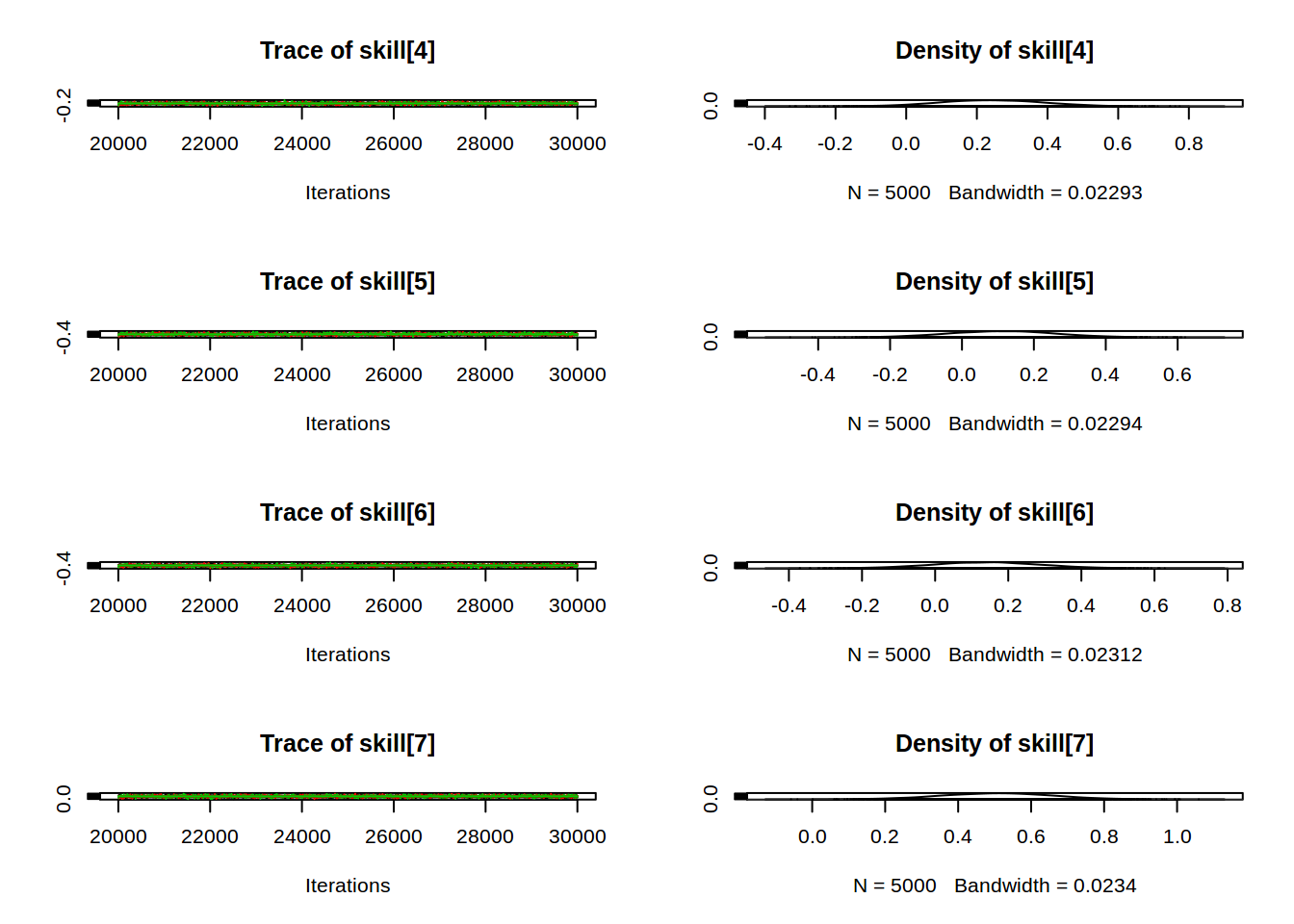
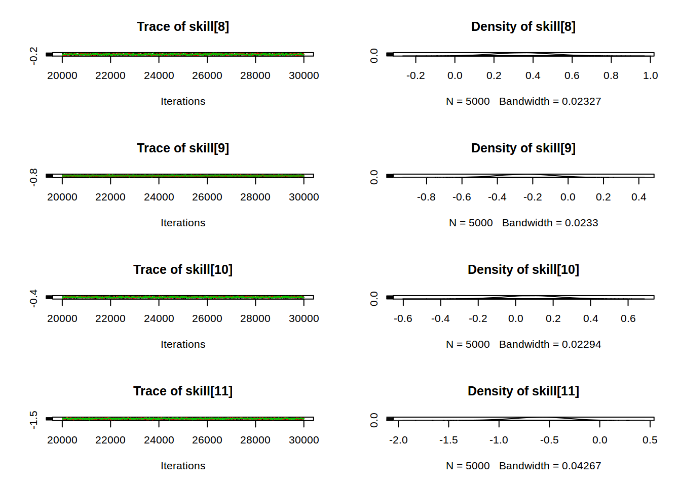
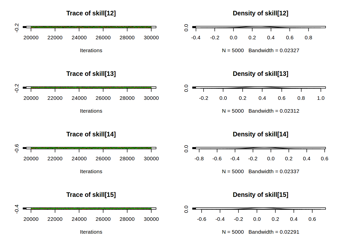
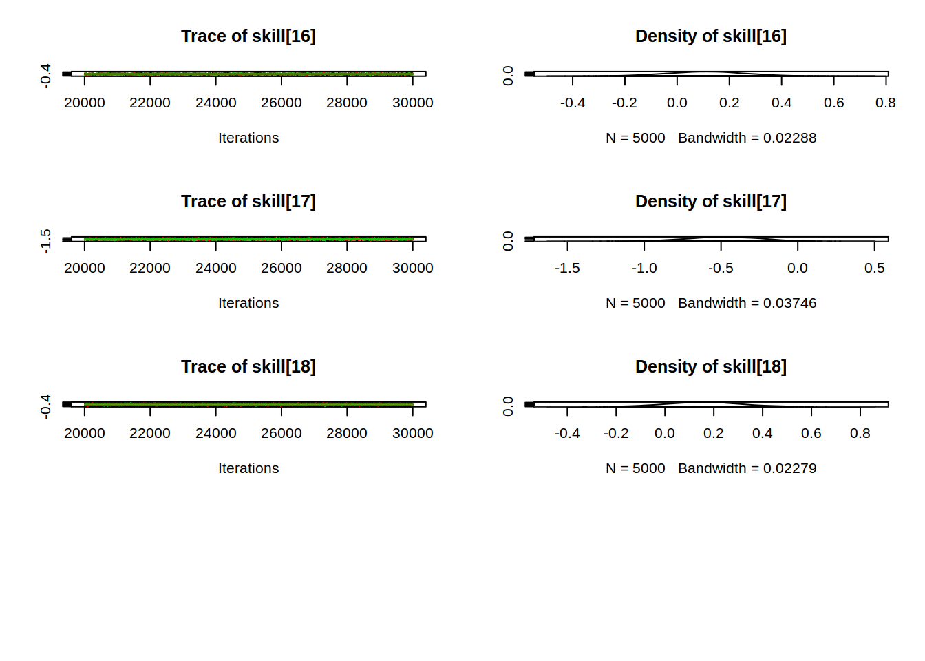

The diagnostics generally look pretty good (although it can be hard to tell from the scaled down images above), with all parameters reaching a satisfactory convergence. The parameter values seem seasonable too, with $\alpha$, $\beta_{hw}$ and $\beta_{aw}$ having mean values close to the MLEs. The differences, for example the baseline having a mean here of around 0.35 compared to 0.23 from the MLE, can be ascribed to including additional team skill parameters.
Assessing fit
Let’s assess model fit further by estimating its accuracy on the
training set. This requires a function to predict a given match,
similarly to how caret provides a predict method for each learning
algorithm.
The first step is to extract the samples of the parameters for future use.
ms <- as.matrix(s)
The team skill intercepts are integer-indexed, so we’ll define a helper function to extract the appropriate column for a given team name.
team_col <- function(team) {
    index <- which(teams == team)
    paste0("skill[", index, "]")
}
Another helper function is the logistic function.
logistic <- function(x) 1 / (1 + exp(-x))
Calculating the match probabilities from parameters simply involves calculating the linear predictor specified in the JAGS model and then drawing from the Bernouilli trial with the resulting estimated probability. I don’t see much difference with either reporting the parameter $p$ as the output of this function or the proportion of Bernouilli trials that were in favour of a home win. The former is more useful when we want an estimate of confidence but for this simple use case the latter will suffice.
predict_match <- function(home, away, hwon, awon) {
    # Form team coefficient
    home_col <- team_col(home)
    away_col <- team_col(away)

    # Calculate lp
    lp <- ms[, 'alpha'] + ms[, home_col] - ms[, away_col] + ms[, "beta_hw"] * (hwon - mean(train_df$hwon)) + ms[, "beta_aw"] * (awon - mean(train_df$awon))

    # Calculate parameter for bernouilli trial
    p <- logistic(lp)

    results <- rbinom(length(p), size=1, prob=p)
    # This gives draws from the distribution, can then obtain probabilities as the proportion of occurrences
    table(results) / length(results)
}
This function returns the predicted probability for each outcome as follows:
predict_match("Melbourne", "Richmond", 3, 2)
## results
##         0         1
## 0.3160667 0.6839333
Without knowing anything about these 2 teams, this prediction that the home team have a significant advantage seems reasonable, particularly since they’ve won all 3 of their last game.s
I’ll just make a wrapper around this to return the outcome with the highest probability to be used to calculate accuracy:
predict_match_outcome <- function(home, away, hwon, awon) {
    probs <- predict_match(home, away, hwon, awon)
    c('n', 'y')[which.max(probs)]
}
predict_match_outcome("Melbourne", "Richmond", 3, 2)
## [1] "y"
Remembering of course that n means away win or draw and y means
home win. It’s ordered in this manner since the aim of the AFL
competition is to predict the home win probability.
Let’s have a look at the training set accuracy then, firstly need to obtain the predicted outcomes for each game in the training set:
train_preds <- apply(train_df, 1, function(row) {
    predict_match_outcome(row[1], row[2],
                          as.numeric(row[3]),
                          as.numeric(row[6])
                          )
})
Leading to an accuracy on the training set of:
mean(train_preds == train_df$outcome2)
## [1] 0.6463292
This is about 3% better than the Naive Bayes and the Boosted Tree classifiers which both got 62% on the training set, but isn’t a huge difference given the increase in model complexity.
A more useful comparison is in terms of the log-loss, which caret
calculates for the benchmark models so I’ll make a quick implementation
here.
logloss <- function(actual, predicted) {
   - (sum(actual * log(predicted) + (1 - actual) * log(1 - predicted))) / length(actual)
}
To use this function we need to calculate the probability estimates of a home win as follows:
train_prob_preds <- apply(train_df, 1, function(row) {
    predict_match(row[1], row[2],
                  as.numeric(row[3]),
                  as.numeric(row[6])
                  )[2] # Extract home win probability
})
# -1 since factors are 1-indexed
logloss(as.numeric(train_df$outcome2)-1, train_prob_preds)
## [1] 0.6264894
Firstly, remember that the log-loss scores output by caret are the
cross-validated score resulting from the optimal parameters and so
aren’t directly comparable to this value above that was calculated from
the entire training set. That said, this value is better than that from
the xgBoost and very similar to the Naive Bayes model. However, as ever,
models can’t be compared on the training set for their predictive value.
Comparison on the test set
A more useful comparison between models is on data that the model hasn’t seen before. In particular ’ll just run a single comparison on the test set. This isn’t ideal; I really should use cross-validation for all models but it’s just far too computationally demanding to use with a Bayesian model fit with JAGS. Also, this test set is relatively small (180 observations), but it’ll do for a rough comparison.
nb_prob_preds <- predict(nb, test_df, type = "prob")[2]  # index to extract home win probs

xgb_prob_preds <- predict(xgb, test_df, type="prob")[2]

bayes_prob_preds <- apply(test_df, 1, function(row) {
    predict_match(row[1], row[2],
                          as.numeric(row[3]),
                          as.numeric(row[6])
                          )[2]
})
lapply(list('nb'=nb_prob_preds, 'xgb'=xgb_prob_preds, 'bayes'=bayes_prob_preds),
       function(preds) logloss(as.numeric(test_df$outcome2)-1, preds))
## $nb
## [1] 0.6037337
##
## $xgb
## [1] 0.6200396
##
## $bayes
## [1] 0.6056966
Surprisingly, the fully hierarchical Bayesian model and the Naive Bayes model which only uses measures of form perform extremely similarly. I would have expected the addition of the team skill levels to enable the Bayesian model to produce more accurate estimates.
Let’s compare the models using the standard accuracy measure:
nb_preds <- predict(nb, test_df)

xgb_preds <- predict(xgb, test_df)

bayes_preds <- apply(test_df, 1, function(row) {
    predict_match_outcome(row[1], row[2],
                          as.numeric(row[3]),
                          as.numeric(row[6])
                          )
})
lapply(list('nb'=nb_preds, 'xgb'=xgb_preds, 'bayes'=bayes_preds),
       function(preds) mean(preds == test_df$outcome2))
## $nb
## [1] 0.6944444
##
## $xgb
## [1] 0.6666667
##
## $bayes
## [1] 0.6777778
As with the log-loss comparison, the Naive Bayes model is rated as the most accurate. An interesting point to make is that all 3 models performed better on the test set than the training data, according to both evaluation criteria. We would not expect this to be the case, and so it hints that this particular test set isn’t representative of the data. This could also be related to the small sample size of this test set.
Given these two results, which model would we choose to use for the final application? This highlights the importance of being aware of how your model will be used. For example, in the AFl prediction league, the models are assessed by information gain, which is a similar function to logloss, and so I will choose models that performed well on this criteria. In other situations, particularly those with unequal costs, Receiver Operating Characteristics may be more appropriate. Accuracy is useful in terms of being easy to understand and relate to, but often it can be misleading, particularly when the classes are imbalanced. In this situation Cohen’s Kappa is a useful statistic.
Conclusions
Despite the fully Bayesian model not having the best logloss on the test set, I’m going to use it for the AFL predictions. I shouldn’t read too much into the results of one (potentially unreliable) test set and the Bayesian model was best on the training set. Again, it’d be ideal to compare these models under cross-validation but JAGS’ long fitting time renders this unfeasible.
I hope this short guide has provided a brief tutorial on using JAGS, as well as sports forecasting. This AFL prediction competition is an interesting case study as the data set is already provided, which saves the effort of manually scraping it. It does, however, tend to restrict you to using predictors already available. For sports that I have more of an understanding of, such as (real) football, I am aware of what other factors could be useful to include. However, there always runs the risk of adding too many inputs for what is a very noisy problem and thereby allowing models to overfit easily. This is where effective diagnostics are required, particularly in visualising the difference between the training and test set, although this is not something I’ve covered in this article.