I’ve recently decided to start using Sweave for producing my publications since I already use R for the data analysis side and LaTeX for the markup, so it seems natural to combine them. In a nutshell, Sweave lets you embed R output directly into your documents, allowing for a more organised workflow. You mark a section as containing R code, then run your analyses with your output, be it in the form of text, a table, or a chart, formatted directly into LaTeX markup. This means that if you need to change your data analysis at all, by using an updated csv of results, or analysing a different group of responses, you just make the required change and when you next compile it all your document will have the updated values/table/chart already in it, rather than having to copy/paste values over or mess around with multiple copies of plots. This provides a much more dynamic working environment, and is especially useful when you come to look back at your publication at a later date and wondered exactly what analysis was done to produce those fantastic looking plots you had, with Sweave and provided you’ve kept your original data file, you can reproduce it exactly.
Setup
The Sweave environment requires an R and a LaTeX package, but handily these come pre-installed with their respective environments. Rather than working in a .tex file as with normal LaTeX you edit a .Rnw file which will contain your R code alongside your LaTeX markup. This file is then compiled with the R output evaluated into standard tex, resulting in a .tex file which can be compiled to dvi/pdf in the usual way. There’s lots of guides out there on setting it up, but my preferred method is to create a simple R makefile, call it make_sweave.R which contains the following line:
Sweave("../path/to/document.Rnw")
Then just call this script first from inside your make file. I tend to use a straight forward bash script rather than a proper makefile, which means that I’m compiling unnecessarily when I haven’t made any changes to my citations but ah well.
Rscript make_sweave.R
pdflatex document
pdflatex document
bibtex document
pdflatex document
pdflatex document
I’ve tended to use Sweave most for automatically generating tables from R dataframes at the moment so I’ll give a short guide on how to do that.
Basic Table
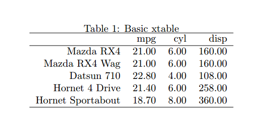
To denote in your .Rnw file that you’re about to input some R code, you use a <<>>= command, with any optional arguments going inbetween the double inequalities, then @ once you’re done. In the example below the first argument is a label I’ve given this snippet for easier referencing, then a named parameter to stop echos from being compiled into the tex file and confirmation that I want the output to be formatted as tex (you can also select html here). The library that we will use to produce tex tables from R dataframes is called xtable and again, it’s included by default in the R standard library. This first example uses the standard mtcars dataset, and will limit it to the first 5 cars and the first 3 columns (mpg, cyl, and disp).
<<first_table, echo=FALSE,results=tex>>=
library(xtable)
df <- mtcars[c(1:5), c(1:3)]
print(xtable(df,
             caption="Basic xtable",
             label="table:mtcars"),
      include.rownames=TRUE,
      caption.placement="top"
      )
@
The xtable function takes in a dataframe as well as optional arguments to supply the caption and LaTeX label of the output table. This is also where you can change the column alignment although we’ll stick with the default for now. The print.xtable function handles the outputting of the xtable object to a tex environment. There are a lot of optional arguments to change parameters such as the floating environment, formatting, placement and so on. The mtcars dataset has the name of the cars as the rownames rather than in a separate column so we’ll tell xtable to print these, although generally I don’t name the rows and so have this option set to False. For some odd reason the default caption placement of an xtable is below the table, whereas in academic publications it should always be on top, here’s where we control this.
This small section of code outputs a table as such:
Neatening it up
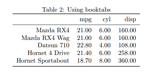
How easy was that! This table looks fine, although it’s a bit crowded. The booktabs LaTeX package makes tables look neater with better padding and whitespace control. Xtable lets you use it with an optional argument to the print call as follows. Note that for this to work you’ll need to install the LaTeX booktabs package and include it with \usepackage{booktabs} in your .Rnw document.
<<second_table, echo=FALSE,results=tex>>=
print(xtable(df,
             caption="Using booktabs",
             label="table:mtcars2"),
      include.rownames=TRUE,
      caption.placement="top",
      booktabs=TRUE
      )
@
Much tidier!
Bolding maximum values
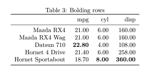
A common pattern in Scientific publications is to bold the maximum value of a row or column to allow for easier reading. Without Sweave you would have to do this manually, locating the maximal values by eye and then tediously placing those cells in bold. If your analysis changed resulting in a different results distribution you’d have to redo all this. I found a handy little function from GitHub user floybix which will do the bolding for you, you just need to tell if it needs to look in columns or rows.
<<third_table, echo=FALSE,results=tex>>=
source("xtable_printbold.R")
printbold(xtable(df,
             caption="Bolding rows",
             label="table:mtcars3"),
      include.rownames=TRUE,
      caption.placement="top",
      booktabs=TRUE,
      each="column"
      )
@
Note that I’ve included this function from a separate source file which needed included. The each optional argument determines whether the maximum values are to be located across rows or columns. We’re still using the mtcars data for now and so are looking for the cars with the maximum number of cylinders, mpg, and engine displacement. This produces the following table, with the maximum column values automatically bolded.
Formatting mean +- standard deviation
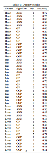
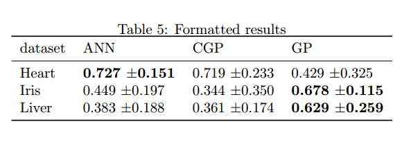
The final part of this guide is more specific to my area of research, comparing machine learning classifiers on various datasets. First I’ll create a dummy data frame with results from Multi-layer Perceptrons (ANN), Genetic Programming (GP), and Cartesian Genetic Programming (CGP) classifiers, run multiple times (as these are stochastic algorithms) on 3 standard datasets from the UCI repository. I’ve also printed this data frame just to visualise this setup.
<<algorithms, echo=FALSE,results=tex>>=
df.cls <- data.frame(dataset=rep(c("Iris", "Heart", "Liver")),
                     algorithm=rep(c("ANN", "GP", "CGP"), each=15),
                     run=rep(seq(5), each=3),
                     accuracy=runif(45))
print(xtable(df.cls[with(df.cls, order(dataset)), ],
             caption="Dummy results",
             label="table:results"),
      caption.placement="top",
      include.rownames=FALSE
      )
@
Most of my experiments result in data frames like this and so I commonly need to take the mean accuracy from each algorithm across all the runs from a dataset and compare these in a table. I made a little function which extends the boldtable snippet described above, which takes a data frame with a blocking factor, a grouping factor and multiple runs on each level of the blocking factor. It returns a new data frame with the average scores written as mean +- standard deviation, and the highest mean score per group bolded.
<<formatted, echo=FALSE,results=tex>>=
source("formattedtable.R")
df.cls.form <- formattedtable(df.cls, "dataset", "algorithm", "accuracy")
print(xtable(df.cls.form,
             caption="Formatted results",
             label="table:formatted_results"),
      caption.placement="top",
      include.rownames=FALSE,
      booktabs=TRUE,
      sanitize.text.function=identity
      )
@
This generates a table as below.
I hope this helped provide a useful insight into what Sweave is, how it works, and how to use it to produce publication quality tables from real world results. I’ve attached the source code to this post and have uploaded the formattables function to GitHub.
